


Time-Dependent Coupling Depth (Codillo et al.)#
Codillo et al., Journal of Geophysical Research (revised version, submitted) modified the base of models of Wilson & van Keken, PEPS, 2023 (II) (as reproduced in FEniCS-SZ) by including a time-dependent coupling depth. Here we derive a new class for these cases and demonstrate their accuracy compared to the original models of Codillo et al.
Model Setup#
As usual we start by adding the path to the modules in the python folder to the system path (so we can find the our earlier modules).
import sys, os, shutil
basedir = ''
if "__file__" in globals(): basedir = os.path.dirname(__file__)
sys.path.insert(0, os.path.join(basedir, os.path.pardir, os.path.pardir, os.path.pardir, 'python'))
Because Codillo et al. considered a time-dependent model with a disclocation creep rheology we will load that class to use as a base.
from fenics_sz.sz_problems.sz_tdep_dislcreep import TDDislSubductionProblem
import fenics_sz.utils
We also require a few other modules and set up output and data folders.
import numpy as np
import pathlib
output_folder = pathlib.Path(os.path.join(basedir, "output"))
output_folder.mkdir(exist_ok=True, parents=True)
data_folder = pathlib.Path(os.path.join(basedir, "data"))
data_folder.mkdir(exist_ok=True, parents=True)
TDGDH1DislSubductionProblem & TDCDGDH1DislSubductionProblem classes#
We derive a new time-dependent subduction model. To match the implementation in Codillo et al. this requires:
a class that uses a GDH1 incoming slab temperature boundary condition rather than the default error function formulation
a class that in addition to using GDH1 boundary condition also has a time-dependent boundary condition on the slab top for the wedge velocity
We implement the first by deriving the TDGDH1DislSubductionProblem class from our previous implementation (TDDislSubductionProblem) and overloading the T_trench member function.
class TDGDH1DislSubductionProblem(TDDislSubductionProblem):
    # Overload the T_trench boundary condition function
    def T_trench(self, x):
        """
        Return temperature at the trench. Use GDH1 from Stein&Stein, Nature, 1992.
        """
        # a few GDH1 parameters
        pi2=np.pi*np.pi
        H_GDH1  = 95.0 # scale depth is 95 km
        T0_GDH1 = 1450.0 # full T in C at base of lithosphere
        kappa_GDH1 = 3.1/(3300.0*1250.0)
        v_GDH1 = fenics_sz.utils.mmpyr_to_mps(10) # 1 cm/yr model velocity in SI
        x_GDH1 = 10*self.A # in m distance from trench assuming 1 cm/yr speed
        x_norm = x_GDH1/H_GDH1 # normalized distance
        Pe_GDH1 = v_GDH1*H_GDH1*1e3/(2*kappa_GDH1) # Peclet number

        # calculate offset in depth due to bathymetry
        deltazsurface = np.minimum(np.maximum(self.deltaztrench*(1.0 - x[0,:]/max(self.deltaxcoast, np.finfo(float).eps)), 0.0), self.deltaztrench)

        # build T_GDH1 with adiabat assumed
        z  = -(x[1,:]+deltazsurface)
        z_norm = z / H_GDH1
        GDH1=z_norm # initial term is normalized conductive state
        for n in range(1,100):
            c = 2.0/(n*np.pi)
            beta = np.sqrt(Pe_GDH1*Pe_GDH1 + n*n*pi2)-Pe_GDH1
            GDH1=GDH1+c*np.exp(-beta*x_norm)*np.sin(n*np.pi*z_norm)
        T_GDH1=GDH1*T0_GDH1 # convert to C
        # add adiabat below Z_GDH1
        T_GDH1 = np.where(z<=H_GDH1,T_GDH1,T0_GDH1+0.3*(z-H_GDH1))

        # return T_GDH1 with the adiabat subtracted out again but this time globally
        return self.Ts + T_GDH1 - z*0.3
Having implemented a GDH1 temperature boundary condition we derive a further TDCDGDH1DislSubductionProblem class (from TDGDH1DislSubductionProblem) that additionally overloads the wv_slabtop member function and indicates that the corresponding boundary condition is time-dependent.
class TDCDGDH1DislSubductionProblem(TDGDH1DislSubductionProblem):
    def members(self):
        # initialize the standard members in the parent class
        super().members()

        # add additional parameter for time-dependent coupling
        self.allowed_input_parameters += ["cd0", "cdf", "dcd", "tc0", "tcf"]
        self.required_parameters += ["cd0", "cdf", "dcd", "tc0", "tcf"]
        self.required_parameters += ["As"] # this was previously only required if oceanic

        self.cd0 = None # initial coupling depth
        self.cdf = None # final coupling depth
        self.dcd = None # partial coupling depth offset
        self.tc0 = None # time for initial coupling (in Myr)
        self.tcf = None # time for full coupling (in Myr)

        # provide a list of boundary conditions that should be evaluated in the time-loop
        self.tdep_bcs = ['vw_slabtop']

    # Overload the vw_slabtop boundary condition function
    def vw_slabtop(self, x):
        """
        Return the wedge velocity on the slab surface as a function of time
        """
        # work out the current coupling depth from the time
        pcd = min(max(self.cd0, self.cd0 + (self.cdf - self.cd0)/(self.tcf - self.tc0)*(self.t_Myr - self.tc0)), self.cdf)
        cd = pcd + self.dcd # current partial coupling depth
        v = np.empty((self.gdim, x.shape[1]))
        for i in range(x.shape[1]):
            v[:,i] = min(max(-(x[1,i]+pcd)/self.dcd, 0.0), 1.0)*self.Vs_nd*self.geom.slab_spline.unittangentx(x[0,i])
        return v
Simulation#
Having set up new classes we can running the simulation on the Izu subduction zone as described in Codillo et al.
Preamble#
Loading everything we need from sz_problem and also set our default plotting and output preferences.
from fenics_sz.sz_problems.sz_params import allsz_params, default_params
from fenics_sz.sz_problems.sz_slab import create_slab, plot_slab
from fenics_sz.sz_problems.sz_geometry import create_sz_geometry
import numpy as np
import dolfinx as df
import pyvista as pv
import requests
import hashlib
import zipfile
import matplotlib.pyplot as pl
Parameters#
We first select the name (“43_Izu”) and resolution scale, resscale and target Courant number cfl of the model.
Resolution
By default the resolution (both spatial and temporal) is low to allow for a quick runtime and smaller website size. If sufficient computational resources are available set a lower resscale and a lower cfl to get higher spatial and temporal resolutions respectively. This is necessary to get results with sufficient accuracy for scientific interpretation.
name = "43_Izu"
resscale = 3
cfl      = 3.0
Then load the remaining parameters from the global suite.
szdict = allsz_params[name]
Codillo et al. used a longer integration time and a higher mantle potential temperatures so we modify those parameters here.
szdict['As'] = 52 # Myr
szdict['Tm'] = 1421.5
szdict['Ac'] = 82 # Myr, final age of overriding lithosphere
And examine the parameters to check.
print("{}:".format(name))
print("{:<20} {:<10}".format('Key','Value'))
print("-"*85)
for k, v in allsz_params[name].items():
    if v is not None and k not in ['z0', 'z15']: print("{:<20} {}".format(k, v))
43_Izu:
Key                  Value
-------------------------------------------------------------------------------------
coast_distance       235
extra_width          12.5
lc_depth             30
io_depth             184
dirname              43_Izu
As                   52
Ac                   82
A                    100.0
sztype               oceanic
Vs                   45.6
xs                   [0, 32.0, 86.0, 138.0, 178.1, 180.8, 199.0, 268.0, 327.5]
ys                   [-6, -15.0, -30.0, -50.0, -80.0, -82.5, -100.0, -175.0, -240.0]
Tm                   1421.5
Setup#
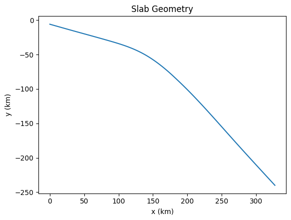
As with other examples in the global suite we start by setting up a slab.
slab = create_slab(szdict['xs'], szdict['ys'], resscale, szdict['lc_depth'])
_ = plot_slab(slab)
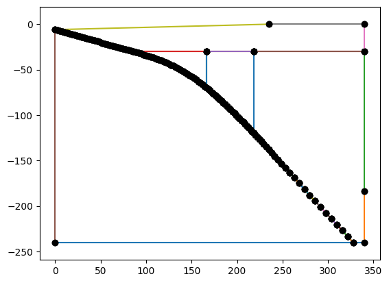
Then we create the subduction zome geometry around the slab.
geom = create_sz_geometry(slab, resscale, szdict['sztype'], szdict['io_depth'], szdict['extra_width'],
                             szdict['coast_distance'], szdict['lc_depth'], szdict['uc_depth'])
_ = geom.plot()
Finally, we declare instances of the TDGDH1DislSubductionProblem and TDCDGDH1DislSubductionProblem problem classes using the dictionary of parameters we loaded and modified above.
sz_gdh1 = TDGDH1DislSubductionProblem(geom, **szdict)
In addition to the parameters stored in the szdict dictionary, our new time-dependent coupling depth class requires some additional parameters, which we add as key word arguments here:
cd0- the initial coupling depth (30 km here)cdf- the final coupling depth (80 km here)dcd- the gap between the partial and full coupling depths (2.5 km here, as indefault_params)tc0- the initial time that the coupling depth starts moving (0 Myr here, the beginning of the simulation)tcf- the end fo coupling depth movement (52 Myr here, the end of the simulation)
sz_tdcd = TDCDGDH1DislSubductionProblem(geom, **szdict,
                                        cd0=30, cdf=80, dcd=default_params['coupling_depth_range'],
                                        tc0=0.0, tcf=szdict['As'])
Solve#
Finally, we choose the timestep to output at integer number of timesteps.
# save period
save_period = 1.0

# Select the timestep based on the approximate target Courant number
dt = cfl*resscale/szdict['Vs']
# Reduce the timestep to get an integer number of timesteps per save period
dt = save_period/np.ceil(save_period/dt)
And run the fixed coupling depth (GDH1) model.
solutions_gdh1 = sz_gdh1.solve(szdict['As'], dt, theta=0.5, rtol=1.e-1, verbosity=1, save_period=save_period)
Entering timeloop with 312 steps (dt = 0.166667 Myr, final time = 52 Myr)
Finished timeloop after 312 steps (final time = 52 Myr)
solutions_tdcd = sz_tdcd.solve(szdict['As'], dt, theta=0.5, rtol=1.e-1, verbosity=1, save_period=save_period)
Entering timeloop with 312 steps (dt = 0.166667 Myr, final time = 52 Myr)
Finished timeloop after 312 steps (final time = 52 Myr)
Plot#
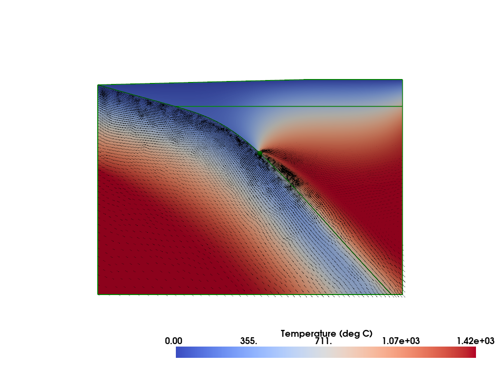
As in previous examples, we can easily plot the solution at the finish time.
First the GDH1 solution.
plotter = pv.Plotter()
fenics_sz.utils.plot.plot_scalar(sz_gdh1.T_i, plotter=plotter, scale=sz_gdh1.T0, gather=True, cmap='coolwarm', scalar_bar_args={'title': 'Temperature (deg C)', 'bold':True})
fenics_sz.utils.plot.plot_vector_glyphs(sz_gdh1.vw_i, plotter=plotter, gather=True, factor=0.1, color='k', scale=fenics_sz.utils.mps_to_mmpyr(sz_gdh1.v0))
fenics_sz.utils.plot.plot_vector_glyphs(sz_gdh1.vs_i, plotter=plotter, gather=True, factor=0.1, color='k', scale=fenics_sz.utils.mps_to_mmpyr(sz_gdh1.v0))
geom.pyvistaplot(plotter=plotter, color='green', width=2)
cdpt = slab.findpoint('Slab::FullCouplingDepth')
fenics_sz.utils.plot.plot_points([[cdpt.x, cdpt.y, 0.0]], plotter=plotter, render_points_as_spheres=True, point_size=10.0, color='green')
fenics_sz.utils.plot.plot_show(plotter)
fenics_sz.utils.plot.plot_save(plotter, output_folder / "{}_td_solution_resscale_{:.2f}_cfl_{:.2f}.png".format(name, resscale, cfl,))
2026-07-15 03:32:52.644 ( 283.671s) [ 7FDAF313B140]vtkXOpenGLRenderWindow.:1416 WARN| bad X server connection. DISPLAY=:99
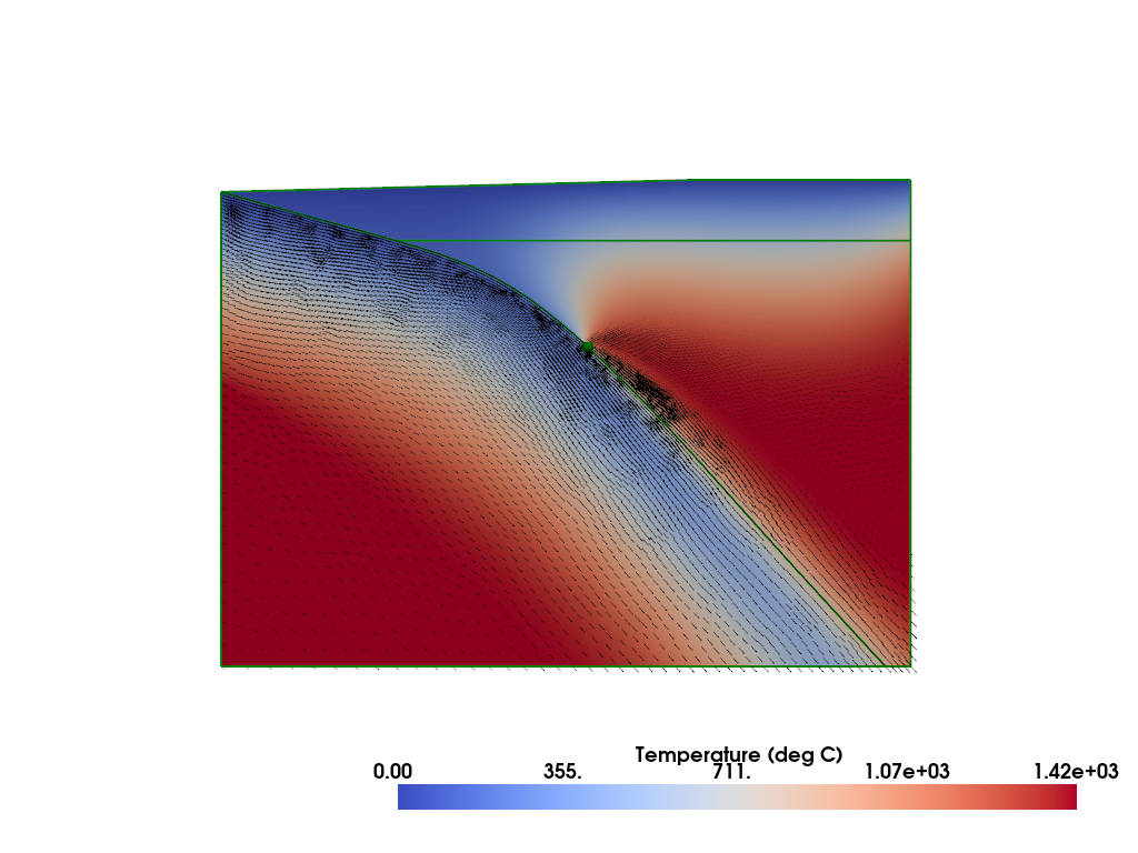
Then the case with a time-dependent coupling depth.
plotter = pv.Plotter()
fenics_sz.utils.plot.plot_scalar(sz_tdcd.T_i, plotter=plotter, scale=sz_tdcd.T0, gather=True, cmap='coolwarm', scalar_bar_args={'title': 'Temperature (deg C)', 'bold':True})
fenics_sz.utils.plot.plot_vector_glyphs(sz_tdcd.vw_i, plotter=plotter, gather=True, factor=0.1, color='k', scale=fenics_sz.utils.mps_to_mmpyr(sz_tdcd.v0))
fenics_sz.utils.plot.plot_vector_glyphs(sz_tdcd.vs_i, plotter=plotter, gather=True, factor=0.1, color='k', scale=fenics_sz.utils.mps_to_mmpyr(sz_tdcd.v0))
geom.pyvistaplot(plotter=plotter, color='green', width=2)
cdpt = slab.findpoint('Slab::FullCouplingDepth')
fenics_sz.utils.plot.plot_points([[cdpt.x, cdpt.y, 0.0]], plotter=plotter, render_points_as_spheres=True, point_size=10.0, color='green')
fenics_sz.utils.plot.plot_show(plotter)
fenics_sz.utils.plot.plot_save(plotter, output_folder / "{}_td_solution_resscale_{:.2f}_cfl_{:.2f}.png".format(name, resscale, cfl,))
We can also save both to disk so that it can be examined with other visualization software (e.g. Paraview).
filename = output_folder / "{}_codillo_gdh1_solution_resscale_{:.2f}_cfl_{:.2f}.bp".format(name, resscale, cfl,)
with df.io.VTXWriter(sz_gdh1.mesh.comm, filename, [sz_gdh1.T_i, sz_gdh1.vs_i, sz_gdh1.vw_i]) as vtx:
    vtx.write(0.0)
# zip the .bp folder so that it can be downloaded from jupyter lab
_ = shutil.make_archive(str(filename), 'zip', root_dir=str(filename.parent), base_dir=str(filename.name))
filename = output_folder / "{}_codillo_tdcd_solution_resscale_{:.2f}_cfl_{:.2f}.bp".format(name, resscale, cfl,)
with df.io.VTXWriter(sz_tdcd.mesh.comm, filename, [sz_tdcd.T_i, sz_tdcd.vs_i, sz_tdcd.vw_i]) as vtx:
    vtx.write(0.0)
# zip the .bp folder so that it can be downloaded from jupyter lab
_ = shutil.make_archive(str(filename), 'zip', root_dir=str(filename.parent), base_dir=str(filename.name))
Plot and save slab temperatures over time#
One of the key outputs of the models in Codillo et al. are the time-dependent variations in the near-slab temperature as seen along paths running subparallel to the slab surface. In Codillo et al. these were obtained using the independent Sepran finite element software. Here we will construct these same paths and compare them to the published solution.
To do this we will need to evaluate the temperature (and lithostatic pressure) along various paths subparallel to the slab surface.
We begin by getting some parameters from the slab surface, firstly its bounding box coordinates.
# slab bounding box
x0 = slab.x[0]
y0 = slab.y[0]
xf = slab.x[-1]
yf = slab.y[-1]
We then evaluate the coordinates of the piecewise linear representation of the slab spline.
# vertices
scoords = [(slab.interpcurves[0].points[0].x, slab.interpcurves[0].points[0].y, 0.0)]
scoords += [(curve.points[-1].x, curve.points[-1].y, 0.0) for curve in slab.interpcurves]
scoords = np.asarray(scoords).transpose()  # transpose now to avoid some issues later
As well as the unit normals to the slab surface.
# normals
snormals = np.stack([-slab.cs(scoords[0,:], nu=1), np.ones(scoords.shape[1]), np.zeros(scoords.shape[1])], axis=0)
snormags = np.sqrt(np.sum(snormals**2, axis=0))
snormals = snormals/snormags
The sediment thicknesses are defined at the trench and at 15 km depth. Between these depths the sediment thickness varies linearly.
Below 15 km depth, the sediment thickness is assumed constant. We can get the sediment thicknesses from szdict and evaluate the piecewise linear sediment thicknesses along the slab surface.
z0  = szdict['z0']  # thickness of sediment at trench
z15 = szdict['z15'] # thickness of sediment at 15km depth

# calculate sediment thicknesses assuming a linear decrease between z0 and z15
y = scoords[1,:]
ssthicks = np.where(y>y0, z0, np.where(y<-15, z15, (z0-z15)*(y-y0)/(y0+15) + z0))
Here we follow the naming convention of Codillo et al. (and Wilson & van Keken, PEPS, 2023 (II)) for the labeling of the paths subparallel to the slab surface (along which temperature and lithostatic pressure are evaluated):
“98”: is the slab surface (and the top of the sediments)
“97”: 0.5 km above (in the mantle wedge and over-riding plate) and parallel to the slab surface (“98”)
“88”-“96”: 1 km increments above (in the mantle wedge and over-riding plate) and parallel to “97” (so “88” and “96” are 9.5 km above and 1.5 km above the slab surface, “98”, respectively)
“99”: below and subparallel to the slab surface (“98”), halfway through the sediments
“100”: below and subparallel to the slab surface (“98”), the base of the sediments
“101”: 0.15 km below and parallel to the base of the sediments (“100”)
“102”: 0.45 km below and parallel to the base of the sediments (“100”)
“103”: 1.4 km below and parallel to the base of the sediments (“100”)
“104”-“112”: 1 km increments below and parallel to “100” (so “104” and “112” are 2.5 km and 10.5 km below the base of the sediments, “100”, respectively)
To achieve this we set up a dictionary of layers along which we will evaluate the temperature in our models. These layers are described by their name (as listed above) and their offset from the slab surface, which is a linear function of the sediment thickness (requiring a sediment factor and a constant offset).
# layer names used in output of Codillo et al. (88 -> 113)
layer_names = [name for name in range(88, 113)]
# factor by which the sediment layer thickness should be multiplied
# (first 11 layers are above sediments, 1 is within and remainder are fully below)
layer_factors = [0.0]*11 + [-0.5] + [-1.0]*13
# constant offsets of layers from slab surface (ignoring sediments)
layer_offsets = np.arange(9.5, 0.0, -1).tolist() + [0.0]*3 + [-0.15, -0.45, -1.4] + np.arange(-2.5, -11, -1).tolist()
# combine into a layers dictionary that we can iterate over
layers = {layer_names[i]:(layer_factors[i], layer_offsets[i]) for i in range(len(layer_names))}
In order to compare to the results of Codillo et al. we download their data from zenodo.
# download the Codillo et al. data for the static coupling depth (but using GDH1)
zipbasename_gdh1 = "43_Izu_52Ma"
zipfilename_gdh1 = pathlib.Path(os.path.join(data_folder, zipbasename_gdh1+".zip"))
if not zipfilename_gdh1.is_file():
    zipfileurl = 'https://zenodo.org/records/15837467/files/43_Izu_52Ma.zip'
    r = requests.get(zipfileurl, allow_redirects=True)
    open(zipfilename_gdh1, 'wb').write(r.content)
assert hashlib.md5(open(zipfilename_gdh1, 'rb').read()).hexdigest() == '76e542001b1f513183fd53b0779f6df8'

# download the Codillo et al. data for the time-dependent coupling depth
zipbasename_tdcd = "43_Izu_D30_to_D80"
zipfilename_tdcd = pathlib.Path(os.path.join(data_folder, zipbasename_tdcd+".zip"))
if not zipfilename_tdcd.is_file():
    zipfileurl = 'https://zenodo.org/records/15837467/files/43_Izu_D30_to_D80.zip'
    r = requests.get(zipfileurl, allow_redirects=True)
    open(zipfilename_tdcd, 'wb').write(r.content)
assert hashlib.md5(open(zipfilename_tdcd, 'rb').read()).hexdigest() == 'b14a22f2ac4f5dfaec900ef2ce54c557'
In addition to saving the slab path temperature data to file we will plot some snapshots and compare them to the data we just downloaded (so we unzip those files here).
# layers to plot
plot_layers = [88, 98, 108]
# simulation times to plot the data
plot_times = [26, 40, 50]

# unzip the corresponding files (if available)
for pt in plot_times:
    slabpathfile_gdh1 = os.path.join(zipbasename_gdh1, 'slabpath.{:03d}'.format(pt))
    with zipfile.ZipFile(zipfilename_gdh1, 'r') as zf:
        try:
            zf.extract(slabpathfile_gdh1, path=data_folder)
        except KeyError:
            pass
    slabpathfile_tdcd = os.path.join(zipbasename_tdcd, 'slabpath.{:03d}'.format(pt))
    with zipfile.ZipFile(zipfilename_tdcd, 'r') as zf:
        try:
            zf.extract(slabpathfile_tdcd, path=data_folder)
        except KeyError:
            pass
Finally, we set some density and thickness parameters in order to calculate the lithostatic pressure.
zcrust = sz_gdh1.deltazc if sz_gdh1.sztype == "continental" else 7.0

rhow = 1.0e3
rhoc = sz_gdh1.rhoc*sz_gdh1.rho0 if sz_gdh1.sztype == "continental" else 3.0e3
rhom = sz_gdh1.rhom*sz_gdh1.rho0

g = 9.81 # m/s^2
Now we can:
loop over the layers and calculate the coordinates of the slab path
evaluate the lithostatic pressure (the same for both models)
evaluate the model cells our slab path intersects with (only needs to be done once as the mesh is assumed the same)
loop over the solutions and evaluate the temperatures along the slab path
save those temperature to the output directory
plot the layers and times we requested above
# set up a figure
fig, axs = pl.subplots(nrows=1, ncols=len(plot_times), figsize=(4*len(plot_times), 6))
if len(plot_times) == 1: axs = [axs]
lines = []

# write headers to files
for sol in solutions_tdcd:
    t = sol['t'] # get time
    with open(output_folder / 'codillo_slabpath_gdh1_{:.0f}.txt'.format(t), "w") as f:
        # x y temperature pressure layer_index
        f.write("#x y T P l"+os.linesep)
    with open(output_folder / 'codillo_slabpath_tdcd_{:.0f}.txt'.format(t), "w") as f:
        # x y temperature pressure layer_index
        f.write("#x y T P l"+os.linesep)

# loop over layers
for name, (factor, offset) in layers.items():
    # translate the slab coordinates to the layer location using the sediment thicknesses and the slab normals
    nscoords = scoords + (factor*ssthicks + offset)*snormals
    # mask the coordinates so that they lie within the bounding box of the slab
    nmask = (nscoords[0,:] >= x0) & (nscoords[0,:] <= xf) & (nscoords[1,:] <= y0) & (nscoords[1,:] >= yf)
    nscoords = nscoords[:,nmask].transpose()

    # work out the slab depth
    zslab = np.asarray([-slab.intersectx(x)[1] for x in nscoords[:,0]])
    # and the depth of the surface (bathymetry)
    zsurface = np.minimum(np.maximum(sz_gdh1.deltaztrench*(1.0 - nscoords[:,0]/max(sz_gdh1.deltaxcoast, np.finfo(float).eps)), 0.0), sz_gdh1.deltaztrench)

    # work out the lithostatic pressure in GPa
    lithP = (rhow*zsurface +                             # contribution of water
             rhoc*(np.minimum(zcrust, zslab)-zsurface) + # contribution of crust
             rhom*(np.maximum(0.0, zslab-zcrust)) +      # contribution of overriding mantle above slab
             rhom*(-nscoords[:,1]-zslab))*g/1.e6         # contribution of subducting slab (subtracts contribution if above slab)

    # work out the cell collisions with the mesh for this layer
    cinds, cells = fenics_sz.utils.mesh.get_cell_collisions(nscoords, sz_gdh1.mesh)

    # loop over the solutions
    for sol_gdh1, sol_tdcd in zip(solutions_gdh1, solutions_tdcd):
        t = sol_gdh1['t'] # get time
        assert np.isclose(t, sol_tdcd['t'])
        T_gdh1 = sol_gdh1['T'] # get temperature function for fixed cd
        T_tdcd = sol_tdcd['T'] # get temperature function for time-dep cd

        # evaluate the slab layer temperatures
        Tslabpath_gdh1 = T_gdh1.eval(nscoords, cells)[:,0]
        Tslabpath_tdcd = T_tdcd.eval(nscoords, cells)[:,0]
        # evaluate the adiabatic contribution
        Ta = -0.3*(nscoords[:,1]+zsurface)
        # and add it to the slabpath T
        Tslabpath_gdh1 += Ta
        Tslabpath_tdcd += Ta

        fmt=["%1.3f"]*4 + ["%d"]
        with open(output_folder / 'codillo_slabpath_gdh1_{:.0f}.txt'.format(t), "a") as f:
            np.savetxt(f,
                        np.column_stack( (nscoords[:,0], nscoords[:,1], Tslabpath_gdh1, lithP, np.ones(len(Tslabpath_gdh1),dtype=int)*name)),
                        delimiter=' ',fmt=fmt)
        with open(output_folder / 'codillo_slabpath_tdcd_{:.0f}.txt'.format(t), "a") as f:
            np.savetxt(f,
                        np.column_stack( (nscoords[:,0], nscoords[:,1], Tslabpath_tdcd, lithP, np.ones(len(Tslabpath_tdcd),dtype=int)*name)),
                        delimiter=' ',fmt=fmt)

        ids = np.where(np.isclose(plot_times, t))[0]
        if len(ids) > 0:
            if name in plot_layers:
                slabpathfile_gdh1 = data_folder / pathlib.Path(os.path.join(zipbasename_gdh1, 'slabpath.{:03.0f}'.format(t)))
                slabpathfile_tdcd = data_folder / pathlib.Path(os.path.join(zipbasename_tdcd, 'slabpath.{:03.0f}'.format(t)))
                fsz_i = lithP <= 7
                if slabpathfile_gdh1.is_file():
                    sepran_data = np.loadtxt(slabpathfile_gdh1)
                    lids = np.where(np.isclose(sepran_data[:,4], name))[0]
                    sepran_T = sepran_data[lids, 2]
                    sepran_P = sepran_data[lids, 3]
                    sepran_i = sepran_P <= 7
                    lines.append(axs[ids[0]].plot(sepran_T[sepran_i], sepran_P[sepran_i], 'k-', label='Sepran (fixed cd)')[0])
                    lines.append(axs[ids[0]].plot(Tslabpath_gdh1[fsz_i], lithP[fsz_i], 'r:', label='FEniCS-SZ (fixed cd)')[0])
                if slabpathfile_tdcd.is_file():
                    sepran_data = np.loadtxt(slabpathfile_tdcd)
                    lids = np.where(np.isclose(sepran_data[:,4], name))[0]
                    sepran_T = sepran_data[lids, 2]
                    sepran_P = sepran_data[lids, 3]
                    sepran_i = sepran_P <= 7
                    lines.append(axs[ids[0]].plot(sepran_T[sepran_i], sepran_P[sepran_i], 'b-', label='Sepran (t-dep cd)')[0])
                    lines.append(axs[ids[0]].plot(Tslabpath_tdcd[fsz_i], lithP[fsz_i], 'g:', label='FEniCS-SZ (t-dep cd)')[0])
                axs[ids[0]].text(Tslabpath_tdcd[fsz_i][-1], lithP[fsz_i][-1], str(name)+' ', ha='right', va='top')

for ax, pt in zip(axs, plot_times):
    ax.set_title('t = {:.0f} Myr'.format(pt,))
    ax.set_xlabel(r'T ($^\circ$C)')
axs[0].set_ylabel(r'P$_\text{lith}$ (GPa)')
_ = fig.legend([l.get_label() for l in lines[:min(len(lines),4)]])
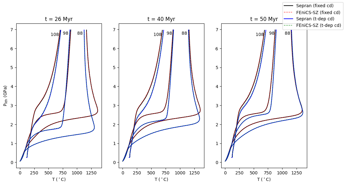
In the figure above we can see a reasonable match between the results from Codillo et al. (“Sepran”) and those generated here (“FEniCS-SZ”). In addition we can see the difference that having time-dependent coupling depth (“t-dep cd”) has on the temperatures in and above the slab compared to a case with a fixed coupling depth (“fixed cd”).
Resolution
Recall that by default the resolution (both spatial and temporal) is low to allow for a quick runtime and smaller website size. If sufficient computational resources are available a lower resscale and cfl should be set above to get the higher spatial and temporal resolutions used by Codillo et al.