Poisson Example 1D

Authors: Kidus Teshome, Cian Wilson

Description

As a reminder we are seeking the approximate solution of the Poisson equation

(20)\[\begin{align} -\frac{d^2 T}{dx^2} &= h % && \text{in }\Omega \end{align}\]

on a 1D domain of unit length, \(\Omega = [0,1]\), where we choose for this example \(h=\frac{1}{4}\pi^2 \sin\left(\frac{\pi x}{2} \right)\). At the boundaries, \(x=0\) and \(x=1\), we apply as boundary conditions

(21)\[\begin{align} T &= 0 && \text{at } x=0 \\ \frac{dT}{dx} &= 0 && \text{at } x=1 \end{align}\]

The first boundary condition is an example of an essential or Dirichlet boundary condition where we specify the value of the solution. The second boundary condition is an example of a natural or Neumann boundary condition that can be interpreted to mean that the solution is symmetrical around \(x\)=1.

The analytical solution to the Poisson equation in 1D with the given boundary conditions and forcing function is simply

(22)\[\begin{equation} T = \sin\left(\frac{\pi x}{2}\right) \end{equation}\]

but we will still solve this numerically as a verification test of our implementation.

Implementation

Traditionally, finite element methods have been implemented using Fortran or C/C++ based codes that, at the core, build the matrix-vector system by numerical integration, after which this system is solved by linear algebraic solvers. Most FEM codes provide options for time-dependence and the ability to solve nonlinear and nonlinearly coupled systems of PDEs. Examples of such codes that have been used in geodynamical applications including subduction zone modeling are ConMan, Sopale, Underworld, CitcomS, MILAMIN, ASPECT, Sepran, Fluidity, and Rhea. A number of these are distributed as open-source software and many among those are currently maintained through the Computational Infrastructure for Geodynamics. These implementations can be shown to be accurate using intercomparisons and benchmarks and make use of advances in parallel computing and efficient linear algebra solver techniques. Yet, modifications to the existing code requires deep insight into the structure of the Fortran/C/C++ code which is not trivial for experienced, let alone beginning, users.

In recent years an alternative approach for FEM has become available which elevates the user interface to simply specifying the FEM problem and solution method with a high-level approach. Python code is used to automatically build a finite element model that can be executed in a variety of environments ranging from Jupyter Notebooks and desktop computers to massively parallel high performance computers. Two prominent examples of this approach are Firedrake and FEniCS. Examples of the use of these two approaches in geodynamical applications are in Davies et al., 2022 and Vynnytska et al., 2013.

Here we will focus on reproducing the results of Wilson & van Keken, 2023 using the latest version of FEniCS, FEniCSx. FEniCS is a suite of open-source numerical libraries for the description of finite element problems. Most importantly it provides a high-level, human-readable language for the description of equations in python using the Unified Form Language (UFL). This is then translated into fast code to assemble the resulting discrete matrix-vector system using the FEniCS Form Compiler (FFC). In Wilson & van Keken, 2023 the following example was presented using FEniCS v2019.1.0 and TerraFERMA, a GUI-based model building framework that also uses FEniCS v2019.1.0. These simulations are publicly available in a zenodo archive and can be run using a docker image.

Preamble

We start by loading all the modules we will require and setting up an output folder.

from mpi4py import MPI
import dolfinx as df
import dolfinx.fem.petsc
import numpy as np
import ufl
import matplotlib.pyplot as pl
import sys, os
basedir = ''
if "__file__" in globals(): basedir = os.path.dirname(__file__)
sys.path.append(os.path.join(basedir, os.path.pardir, os.path.pardir, 'python'))
import utils.mesh
import pathlib
output_folder = pathlib.Path(os.path.join(basedir, "output"))
output_folder.mkdir(exist_ok=True, parents=True)

Solution

We then declare a python function solve_poisson_1d that contains a complete description of the discrete Poisson equation problem.

This function follows much the same flow as described in the introduction

1. we describe the domain \(\Omega\) and discretize it into ne elements or cells to make a mesh

2. we declare the function space, V, to use Lagrange polynomials of degree p

3. we define the Dirichlet boundary condition, bc at \(x=0\), setting the desired value there to be 0

4. we define the right hand side forcing function \(h\), h

5. using the function space we declare trial, T_a, and test, T_t, functions and describe the discrete weak forms, S and f, that will be used to assemble the matrix and vector

6. we assemble and solve the matrix problem using a linear algebra back-end and return the temperature solution, T_i

For a more detailed description of solving the Poisson equation using FEniCSx, see the FEniCSx tutorial.

def solve_poisson_1d(ne, p=1):
    """
    A python function to solve a one-dimensional Poisson problem
    on a unit interval domain.
    Parameters:
      * ne - number of elements
      * p  - polynomial order of the solution function space
    """
    
    # Describe the domain (a one-dimensional unit interval)
    # and also the tessellation of that domain into ne 
    # equally spaced elements
    mesh = df.mesh.create_unit_interval(MPI.COMM_WORLD, ne)

    # Define the solution function space using Lagrange polynomials
    # of order p
    V = df.fem.functionspace(mesh, ("Lagrange", p))

    # Define the location of the boundary, x=0
    def boundary(x):
        return np.isclose(x[0], 0)
    # Specify the value and define a boundary condition (bc)
    boundary_dofs = df.fem.locate_dofs_geometrical(V, boundary)
    gD = df.fem.Constant(mesh, df.default_scalar_type(0.0))
    bc = df.fem.dirichletbc(gD, boundary_dofs, V)

    # Define the right hand side function, h
    x = ufl.SpatialCoordinate(mesh)
    h = (ufl.pi**2)*ufl.sin(ufl.pi*x[0]/2)/4

    # Define the trial and test functions on the same function space (V)
    T_a = ufl.TrialFunction(V)
    T_t = ufl.TestFunction(V)
    
    # Define the integral to be assembled into the stiffness matrix
    S = ufl.inner(ufl.grad(T_t), ufl.grad(T_a))*ufl.dx
    # Define the integral to be assembled into the forcing vector
    f = T_t*h*ufl.dx

    # Compute the solution (given the boundary condition, bc)
    problem = df.fem.petsc.LinearProblem(S, f, bcs=[bc], \
                                         petsc_options={"ksp_type": "preonly", \
                                                        "pc_type": "lu",
                                                        "pc_factor_mat_solver_type": "mumps"})
    T_i = problem.solve()

    # Return the solution
    return T_i

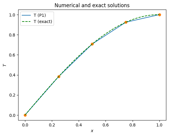
We can then use solve_poisson_1d to solve on, for example, ne = 4 elements with P1, p = 1 elements.

ne = 4
p = 1
T_P1 = solve_poisson_1d(ne, p=p)
T_P1.name = "T (P1)"

In order to visualize the solution, we write a python function that evaluates both the numerical and analytical solutions at a series of points and plots them both using matplotlib.

def plot_1d(T, x, filename=None):
    nx = len(x)
    # convert 1d points to 3d points (necessary for eval call)
    xyz = np.stack((x, np.zeros_like(x), np.zeros_like(x)), axis=1)
    # work out which cells those points are in using a utility function we provide
    mesh = T.function_space.mesh
    cinds, cells = utils.mesh.get_cell_collisions(xyz, mesh)
    # evaluate the numerical solution
    T_x = T.eval(xyz[cinds], cells)[:,0]
    # if running in parallel gather the solution to the rank-0 process
    cinds_g = mesh.comm.gather(cinds, root=0)
    T_x_g = mesh.comm.gather(T_x, root=0)
    # only plot on the rank-0 process
    if mesh.comm.rank == 0:
        T_x = np.empty_like(x)
        for r, cinds_p in enumerate(cinds_g):
            for i, cind in enumerate(cinds_p):
                T_x[cind] = T_x_g[r][i]
        # plot
        fig = pl.figure()
        ax = fig.gca()
        ax.plot(x, T_x, label=T.name)                              # numerical solution
        ax.plot(x[::int(nx/ne/p)], T_x[::int(nx/ne/p)], 'o')       # nodal points (uses globally defined ne and p)
        ax.plot(x, np.sin(np.pi*x/2), '--g', label='T (exact)')    # analytical solution
        ax.legend()
        ax.set_xlabel('$x$')
        ax.set_ylabel('$T$')
        ax.set_title('Numerical and exact solutions')
        # save the figure
        if filename is not None: fig.savefig(filename)

Comparing the numerical, \(\tilde{T}\), and analytical, \(T\), solutions we can see that even at this small number of elements we do a good job at reproducing the correct answer.

x = np.linspace(0, 1, 201)
plot_1d(T_P1, x, filename=output_folder / '1d_poisson_P1_solution.pdf')

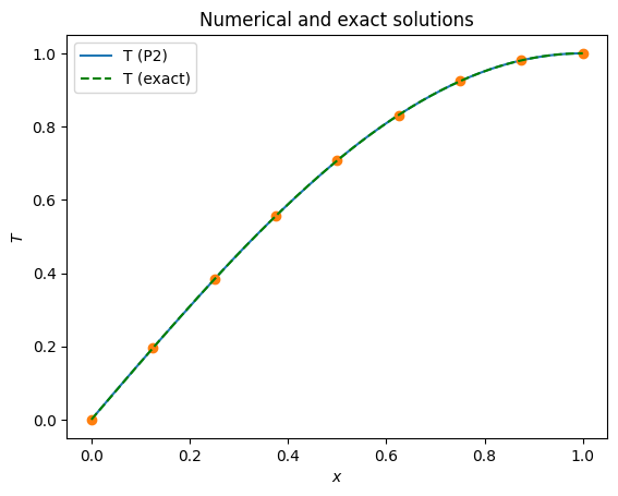
We can also try with a higher order element and see how it improves the solution.

ne = 4
p = 2
T_P2 = solve_poisson_1d(ne, p=p)
T_P2.name = "T (P2)"

The higher polynomial degree qualitatively appears to have a dramatic improvement in the solution accuracy.

x = np.linspace(0, 1, 201)
plot_1d(T_P2, x, filename=output_folder / '1d_poisson_P2_solution.pdf')

Testing

We can quantify the error in cases where the analytical solution is known by taking the L2 norm of the difference between the numerical and exact solutions.

def evaluate_error(T_i):
    """
    A python function to evaluate the l2 norm of the error in 
    the one dimensional Poisson problem given a known analytical
    solution.
    """
    # Define the exact solution
    x  = ufl.SpatialCoordinate(T_i.function_space.mesh)
    Te = ufl.sin(ufl.pi*x[0]/2)
    
    # Define the error between the exact solution and the given
    # approximate solution
    l2err = df.fem.assemble_scalar(df.fem.form((T_i - Te)*(T_i - Te)*ufl.dx))
    l2err = T_i.function_space.mesh.comm.allreduce(l2err, op=MPI.SUM)**0.5
    
    # Return the l2 norm of the error
    return l2err

Repeating the numerical experiments with increasing ne allows us to test the convergence of our approximate finite element solution to the known analytical solution. A key feature of any discretization technique is that with an increasing number of degrees of freedom (DOFs) these solutions should converge, i.e. the error in our approximation should decrease. As an error metric we will use the \(L^2\) norm of the difference between the approximate, \(\tilde{T}\), and analytical, \(T\), solutions

(23)\[\begin{equation} e_{L^2} = \sqrt{\int_\Omega \left(\tilde{T} - T\right)^2 dx} \end{equation}\]

The rate at which this decreases is known as the order of convergence. Numerical analysis predicts a certain order depending on the type of the polynomials used as finite element shape functions and other constraints related to the well-posedness of the problem. For piecewise linear shape functions we expect second-order convergence, that is that the error decreases as \(h^{-2}\) where \(h\) is the nodal point spacing. With piecewise quadratic elements we expect to see third-order convergence.

# Open a figure for plotting
fig = pl.figure()
ax = fig.gca()

# List of polynomial orders to try
ps = [1, 2]
# List of resolutions to try
nelements = [10, 20, 40, 80, 160, 320]
# Keep track of whether we get the expected order of convergence
test_passes = True
# Loop over the polynomial orders
for p in ps:
    # Accumulate the errors
    errors_l2_a = []
    # Loop over the resolutions
    for ne in nelements:
        # Solve the 1D Poisson problem
        T_i = solve_poisson_1d(ne, p)
        # Evaluate the error in the approximate solution
        l2error = evaluate_error(T_i)
        # Print to screen and save if on rank 0
        if T_i.function_space.mesh.comm.rank == 0:
            print('ne = ', ne, ', l2error = ', l2error)
        errors_l2_a.append(l2error)

    # Work out the order of convergence at this p
    hs = 1./np.array(nelements)/p
    
    # Write the errors to disk
    if T_i.function_space.mesh.comm.rank == 0:
        with open(output_folder / '1d_poisson_convergence_p{}.csv'.format(p), 'w') as f:
            np.savetxt(f, np.c_[nelements, hs, errors_l2_a], delimiter=',', 
                        header='nelements, hs, l2errs')
        
    # Fit a line to the convergence data
    fit = np.polyfit(np.log(hs), np.log(errors_l2_a),1)
    
    if T_i.function_space.mesh.comm.rank == 0:
        print("***********  order of accuracy p={}, order={:.2f}".format(p,fit[0]))
    
    # log-log plot of the error  
    ax.loglog(hs,errors_l2_a,'o-',label='p={}, order={:.2f}'.format(p,fit[0]))
    
    # Test if the order of convergence is as expected
    test_passes = test_passes and fit[0] > p+0.9

# Tidy up the plot
ax.set_xlabel('h')
ax.set_ylabel('||e||_2')
ax.grid()
ax.set_title('Convergence')
ax.legend()

# Write convergence to disk
if T_i.function_space.mesh.comm.rank == 0:
    fig.savefig(output_folder / '1d_poisson_convergence.pdf')
    
    print("***********  convergence figure in output/1d_poisson_convergence.pdf")

# Check if we passed the test
assert(test_passes)

ne =  10 , l2error =  0.0015918430698243743
ne =  20 , l2error =  0.00039812153736439715
ne =  40 , l2error =  9.954043481100349e-05
ne =  80 , l2error =  2.4885737309860596e-05
ne =  160 , l2error =  6.221474217276118e-06
ne =  320 , l2error =  1.5553696816469428e-06
***********  order of accuracy p=1, order=2.00

ne =  10 , l2error =  1.57542178485356e-05
ne =  20 , l2error =  1.9698108549866896e-06
ne =  40 , l2error =  2.462430383144762e-07
ne =  80 , l2error =  3.078090082645182e-08
ne =  160 , l2error =  3.8476310988427584e-09
ne =  320 , l2error =  4.809538317037086e-10
***********  order of accuracy p=2, order=3.00

***********  convergence figure in output/1d_poisson_convergence.pdf

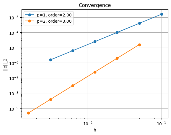
The convergence tests show that we achieve the expected orders of convergence for all polynomial degrees.

Finish up

Convert this notebook to a python module (saving first and ignoring markdown cells and those tagged as “main” or “ipy”).

from ipylab import JupyterFrontEnd
app = JupyterFrontEnd()
app.commands.execute('docmanager:save')
!jupyter nbconvert --TagRemovePreprocessor.enabled=True --TagRemovePreprocessor.remove_cell_tags="['main', 'ipy']" --TemplateExporter.exclude_markdown=True --TemplateExporter.exclude_input_prompt=True --TemplateExporter.exclude_output_prompt=True --NbConvertApp.export_format=script --ClearOutputPreprocessor.enabled=True --FilesWriter.build_directory=../../python/background --NbConvertApp.output_base=poisson_1d 2.2b_poisson_1d.ipynb

[NbConvertApp] Converting notebook 2.2b_poisson_1d.ipynb to script

[NbConvertApp] Writing 4359 bytes to ../../python/background/poisson_1d.py