Steady-State Subduction Zone Setup

Authors: Kidus Teshome, Cian Wilson

Recalling our implementation strategy we are following a similar workflow to that seen in the background examples.

1. we will describe the subduction zone geometry and tesselate it into non-overlapping triangles to create a mesh

2. we will declare function spaces for the temperature, wedge velocity and pressure, and slab velocity and pressure

3. using these function spaces we will declare trial and test functions

4. we will define Dirichlet boundary conditions at the boundaries as described in the introduction

5. we will describe discrete weak forms for temperature and each of the coupled velocity-pressure systems that will be used to assemble the matrices (and vectors) to be solved

6. we will set up matrices and solvers for the discrete systems of equations

7. we will solve the matrix problems

We have now implemented all but the case-specific final step of solving the coupled velocity-pressure-temperature problem. In this notebook we do this for the case of steady-state, isoviscous solutions, deriving a new SteadyIsoSubductionProblem class from the SteadySubductionProblem class we implemented in notebooks/03_sz_problems/3.3a_sz_steady_problem.ipynb.

Preamble

Let’s start by adding the path to the modules in the python folder to the system path (so we can find the our custom modules).

import sys, os
basedir = ''
if "__file__" in globals(): basedir = os.path.dirname(__file__)
sys.path.append(os.path.join(basedir, os.path.pardir, os.path.pardir, 'python'))

Let’s also load the module generated by the previous notebooks to get access to the parameters and functions defined there.

from sz_problems.sz_params import default_params, allsz_params
from sz_problems.sz_slab import create_slab
from sz_problems.sz_geometry import create_sz_geometry
from sz_problems.sz_problem import StokesSolverNest, TemperatureSolver
from sz_problems.sz_steady_problem import SteadySubductionProblem

Then let’s load all the required modules at the beginning.

import geometry as geo
import utils
from mpi4py import MPI
import dolfinx as df
import dolfinx.fem.petsc
from petsc4py import PETSc
import numpy as np
import scipy as sp
import ufl
import basix.ufl as bu
import matplotlib.pyplot as pl
import copy
import pyvista as pv
import pathlib
output_folder = pathlib.Path(os.path.join(basedir, "output"))
output_folder.mkdir(exist_ok=True, parents=True)

SteadyIsoSubductionProblem class

We build on the SteadySubductionProblem class implemented in notebooks/03_sz_problems/3.3a_sz_steady_problem.ipynb, deriving a SteadyIsoSubductionProblem class that solves the equations for a steady-state, isoviscous case.

7. Solution

In the isoviscous case, \(\eta\) = 1 (eta = 1), only the temperature depends on the velocity (and not vice-versa). So to solve the full system of equations we only need to solve the two velocity-pressure systems once (already implemented in SubductionProblem.solve_stokes_isoviscous) before solving the temperature to get a fully converged solution for all variables (implemented below in solve).

class SteadyIsoSubductionProblem(SteadySubductionProblem):
    def solve(self, petsc_options_s=None, petsc_options_T=None):
        """
        Solve the coupled temperature-velocity-pressure problem assuming an isoviscous rheology

        Keyword Arguments:
          * petsc_options_s - a dictionary of petsc options to pass to the Stokes solver 
                              (defaults to an LU direct solver using the MUMPS library) 
          * petsc_options_T - a dictionary of petsc options to pass to the temperature solver 
                              (defaults to an LU direct solver using the MUMPS library) 
        """

        # first solve both Stokes systems
        self.solve_stokes_isoviscous(petsc_options=petsc_options_s)

        # retrieve the temperature forms
        ST, fT, _ = self.temperature_forms()
        solver_T = TemperatureSolver(ST, fT, self.bcs_T, self.T_i, 
                                     petsc_options=petsc_options_T)
        # and solve the temperature problem
        self.T_i = solver_T.solve()

        # only update the pressure at the end as it is not necessary earlier
        self.update_p_functions()

Demonstration - Benchmark case 1

So now we have a full description of the isoviscous problem for an isoviscous steady-state problem and, as before, can demonstrate using a low resolution, resscale = 5.0

resscale = 5.0

with the isoviscous benchmark geometry parameters (as in previous notebooks)

xs = [0.0, 140.0, 240.0, 400.0]
ys = [0.0, -70.0, -120.0, -200.0]
lc_depth = 40
uc_depth = 15
coast_distance = 0
extra_width = 0
sztype = 'continental'
io_depth = 139
A      = 100.0      # age of subducting slab (Myr)
qs     = 0.065      # surface heat flux (W/m^2)
Vs     = 100.0      # slab speed (mm/yr)

We can then use these to instantiate our slab, geometry and SteadyIsoSubductionProblem.

slab = create_slab(xs, ys, resscale, lc_depth)
geom = create_sz_geometry(slab, resscale, sztype, io_depth, extra_width, 
                            coast_distance, lc_depth, uc_depth)
sz_case1 = SteadyIsoSubductionProblem(geom, A=A, Vs=Vs, sztype=sztype, qs=qs)

We can use this to solve for the (now full) solution to benchmark case 1,

sz_case1.solve()

and compare the diagnostics to the benchmark solutions.

diag = sz_case1.get_diagnostics()

print('')
print('{:<12} {:<12} {:<12} {:<12} {:<12} {:<12}'.format('resscale', 'T_ndof', 'T_{200,-100}', 'Tbar_s', 'Tbar_w', 'Vrmsw'))
print('{:<12.4g} {:<12d} {:<12.4f} {:<12.4f} {:<12.4f} {:<12.4f}'.format(resscale, *diag.values()))

T_ndof = 5812
T_(200,-100) = 517.17 deg C
slab_diag_length = 111.80
T_slab = 451.95 deg C
wedge_diag_area = 5500.00
T_wedge = 927.02 deg C
V_rms,w = 34.64 mm/yr

resscale     T_ndof       T_{200,-100} Tbar_s       Tbar_w       Vrmsw       
5            5812         517.1668     451.9452     927.0205     34.6379     

For comparison here are the values reported for case 1 using TerraFERMA in Wilson & van Keken, 2023:

resscale	\(T_{\text{ndof}} \)	\(T_{(200,-100)}^*\)	\(\overline{T}_s^*\)	\( \overline{T}_w^* \)	\(V_{\text{rms},w}^*\)
2.0	21403	517.17	451.83	926.62	34.64
1.0	83935	516.95	451.71	926.33	34.64
0.5	332307	516.86	451.63	926.15	34.64

so even though we are at lower resolution our solution appears to be reasonably good in this case. This is just intended as a demonstration and we will perform more benchmark testing later.

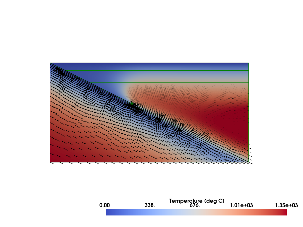
For now, we can plot the temperature and velocity solutions.

plotter_iso = utils.plot.plot_scalar(sz_case1.T_i, scale=sz_case1.T0, gather=True, cmap='coolwarm', scalar_bar_args={'title': 'Temperature (deg C)', 'bold':True})
utils.plot.plot_vector_glyphs(sz_case1.vw_i, plotter=plotter_iso, factor=0.1, gather=True, color='k', scale=utils.mps_to_mmpyr(sz_case1.v0))
utils.plot.plot_vector_glyphs(sz_case1.vs_i, plotter=plotter_iso, factor=0.1, gather=True, color='k', scale=utils.mps_to_mmpyr(sz_case1.v0))
utils.plot.plot_geometry(sz_case1.geom, plotter=plotter_iso, color='green', width=2)
utils.plot.plot_couplingdepth(sz_case1.geom.slab_spline, plotter=plotter_iso, render_points_as_spheres=True, point_size=10.0, color='green')
utils.plot.plot_show(plotter_iso)
utils.plot.plot_save(plotter_iso, output_folder / "sz_problem_case1_solution.png")

The output can also be saved to disk and opened with other visualization software (e.g. Paraview).

filename = output_folder / "sz_problem_case1_solution.bp"
with df.io.VTXWriter(sz_case1.mesh.comm, filename, [sz_case1.T_i, sz_case1.vs_i, sz_case1.vw_i]) as vtx:
    vtx.write(0.0)
# zip the .bp folder so that it can be downloaded from Jupyter lab
zipfilename = filename.with_suffix(".zip")
!zip -r $zipfilename $filename

  adding: output/sz_problem_case1_solution.bp/ (stored 0%)
  adding: output/sz_problem_case1_solution.bp/mmd.0 (deflated 64%)
  adding: output/sz_problem_case1_solution.bp/profiling.json (deflated 62%)
  adding: output/sz_problem_case1_solution.bp/md.idx (deflated 59%)
  adding: output/sz_problem_case1_solution.bp/md.0 (deflated 76%)
  adding: output/sz_problem_case1_solution.bp/data.0 (deflated 67%)

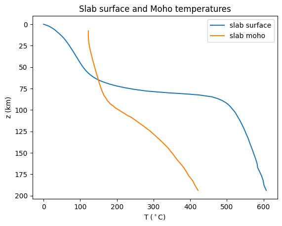
It’s also common to want to interogate the temperature at various points in the domain or along the slab. Here we provide an example function for doing that that plots the slab temperature along the slab surface and along the slab Moho at 7km depth (into the slab).

def plot_slab_temperatures(sz):
    """
    Plot the slab surface and Moho (7 km slab depth)

    Arguments:
      * sz - a solved SubductionProblem instance
    """
    # get some points along the slab
    slabpoints = np.array([[curve.points[0].x, curve.points[0].y, 0.0] for curve in sz.geom.slab_spline.interpcurves])
    # do the same along a spline deeper in the slab
    slabmoho = copy.deepcopy(sz.geom.slab_spline)
    slabmoho.translatenormalandcrop(-7.0)
    slabmohopoints = np.array([[curve.points[0].x, curve.points[0].y, 0.0] for curve in slabmoho.interpcurves])
    # set up a figure
    fig = pl.figure()
    ax = fig.gca()
    # plot the slab temperatures
    cinds, cells = utils.mesh.get_cell_collisions(slabpoints, sz.mesh)
    ax.plot(sz.T_i.eval(slabpoints, cells)[:,0], -slabpoints[:,1], label='slab surface')
    # plot the moho temperatures
    mcinds, mcells = utils.mesh.get_cell_collisions(slabmohopoints, sz.mesh)
    ax.plot(sz.T_i.eval(slabmohopoints, mcells)[:,0], -slabmohopoints[:,1], label='slab moho')
    # labels, title etc.
    ax.set_xlabel('T ($^\circ$C)')
    ax.set_ylabel('z (km)')
    ax.set_title('Slab surface and Moho temperatures')
    ax.legend()
    ax.invert_yaxis()
    return fig

fig = plot_slab_temperatures(sz_case1)
fig.savefig(output_folder / "sz_problem_case1_slabTs.png")

Finish up

Convert this notebook to a python module (saving first and ignoring markdown cells and those tagged as “main” or “ipy”).

from ipylab import JupyterFrontEnd
app = JupyterFrontEnd()
app.commands.execute('docmanager:save')
!jupyter nbconvert --TagRemovePreprocessor.enabled=True --TagRemovePreprocessor.remove_cell_tags="['main', 'ipy']" --TemplateExporter.exclude_markdown=True --TemplateExporter.exclude_input_prompt=True --TemplateExporter.exclude_output_prompt=True --NbConvertApp.export_format=script --ClearOutputPreprocessor.enabled=True --FilesWriter.build_directory=../../python/sz_problems --NbConvertApp.output_base=sz_steady_isoviscous 3.3b_sz_steady_isoviscous.ipynb

[NbConvertApp] Converting notebook 3.3b_sz_steady_isoviscous.ipynb to script

[NbConvertApp] Writing 3313 bytes to ../../python/sz_problems/sz_steady_isoviscous.py