Steady-State Subduction Zone Setup#
Themes and variations - varying the coupling depth#
In this notebook we will try seeing the effect of varying the coupling depth on the benchmark solution.
Preamble#
Let’s start by adding the path to the modules in the python folder to the system path (so we can find the our custom modules).
import sys, os
basedir = ''
if "__file__" in globals(): basedir = os.path.dirname(__file__)
sys.path.insert(0, os.path.join(basedir, os.path.pardir, os.path.pardir, 'python'))
Then load everything we need from sz_problems and other modules.
import fenics_sz.utils
from fenics_sz.sz_problems.sz_params import default_params, allsz_params
from fenics_sz.sz_problems.sz_slab import create_slab
from fenics_sz.sz_problems.sz_geometry import create_sz_geometry
from fenics_sz.sz_problems.sz_steady_isoviscous import SteadyIsoSubductionProblem
from fenics_sz.sz_problems.sz_steady_dislcreep import SteadyDislSubductionProblem
import pathlib
output_folder = pathlib.Path(os.path.join(basedir, "output"))
output_folder.mkdir(exist_ok=True, parents=True)
We will now re-use all of the parameters for case 2
xs = [0.0, 140.0, 240.0, 400.0]
ys = [0.0, -70.0, -120.0, -200.0]
lc_depth = 40
uc_depth = 15
coast_distance = 0
extra_width = 0
sztype = 'continental'
io_depth_2 = 154.0
A      = 100.0      # age of subducting slab (Myr)
qs     = 0.065      # surface heat flux (W/m^2)
Vs     = 100.0      # slab speed (mm/yr)
but vary the coupling depth by passing in an additional keyword argument coupling_depth to create_slab. The rest of the solution procedure is the same as before.
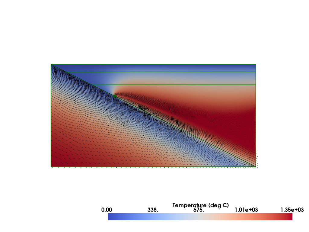
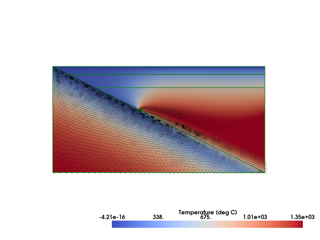
Let’s loop over a series of coupling depths to see how varying it changes the solution.
# set a list of coupling depths to try
coupling_depths = [60.0, 80.0, 100.0]
resscale3 = 3.0

# set up a list to save the diagnostics from each
diagnostics = []
# loop over the couplings depths
for coupling_depth in coupling_depths:
    # create the slab object, all of the input arguments are the same as in case 2
    # but this time we also pass in the coupling_depth keyword argument to override
    # the default value (80 km)
    slab_dc = create_slab(xs, ys, resscale3, lc_depth, coupling_depth=coupling_depth)
    # set up the geometry
    geom_dc = create_sz_geometry(slab_dc, resscale3, sztype, io_depth_2, extra_width,
                                            coast_distance, lc_depth, uc_depth)
    # set up the subduction zone problem
    sz_dc = SteadyDislSubductionProblem(geom_dc, A=A, Vs=Vs, sztype=sztype, qs=qs)

    # solve the steady state problem
    if sz_dc.comm.rank == 0: print(f"\nSolving steady state flow with coupling depth = {coupling_depth}km...")
    sz_dc.solve()

    # retrieve the diagnostics
    diagnostics.append(sz_dc.get_diagnostics())

    # plot the solution
    plotter_dc = fenics_sz.utils.plot.plot_scalar(sz_dc.T_i, scale=sz_dc.T0, gather=True, cmap='coolwarm',
                                   scalar_bar_args={'title': 'Temperature (deg C)', 'bold':True})
    fenics_sz.utils.plot.plot_vector_glyphs(sz_dc.vw_i, plotter=plotter_dc, gather=True, factor=0.05, color='k',
                             scale=fenics_sz.utils.mps_to_mmpyr(sz_dc.v0))
    fenics_sz.utils.plot.plot_vector_glyphs(sz_dc.vs_i, plotter=plotter_dc, gather=True, factor=0.05, color='k',
                             scale=fenics_sz.utils.mps_to_mmpyr(sz_dc.v0))
    sz_dc.geom.pyvistaplot(plotter=plotter_dc, color='green', width=2)
    cdpt = sz_dc.geom.slab_spline.findpoint('Slab::FullCouplingDepth')
    fenics_sz.utils.plot.plot_points([[cdpt.x, cdpt.y, 0.0]], plotter=plotter_dc, render_points_as_spheres=True, point_size=10.0, color='green')
    fenics_sz.utils.plot.plot_show(plotter_dc)
    fenics_sz.utils.plot.plot_save(plotter_dc, output_folder / f"sz_steady_tests_dc{coupling_depth}_solution.png")

    # clean up
    del plotter_dc
    del sz_dc
    del geom_dc
    del slab_dc
Solving steady state flow with coupling depth = 60.0km...
Iteration   Residual     Relative Residual
------------------------------------------
0           15775.6      1
1           2280.97      0.144589
2           396.118      0.0251095
3           162.11       0.010276
4           90.6929      0.00574893
5           58.4212      0.00370326
6           38.4282      0.00243593
7           25.1861      0.00159652
8           16.5768      0.00105079
9           11.0517      0.000700558
10          7.51178      0.000476164
11          5.21931      0.000330847
12          3.70904      0.000235112
13          2.69295      0.000170703
14          1.99333      0.000126355
15          1.50038      9.51078e-05
16          1.14556      7.2616e-05
17          0.885316     5.61193e-05
18          0.691324     4.38223e-05
19          0.544707     3.45284e-05
20          0.432575     2.74205e-05
21          0.345932     2.19283e-05
22          0.278376     1.7646e-05
23          0.225277     1.428e-05
24          0.183232     1.16149e-05
25          0.149717     9.4904e-06
26          0.122835     7.78638e-06
27          0.10115      6.41179e-06
28          0.0835647    5.29708e-06
29 0.0692349 4.38873e-06
Solving steady state flow with coupling depth = 80.0km...
Iteration   Residual     Relative Residual
------------------------------------------
0           14345.4      1
1           2039.1       0.142143
2           297.088      0.0207097
3           115.363      0.00804178
4           59.3975      0.00414053
5           35.4511      0.00247125
6           22.3506      0.00155804
7           14.5106      0.00101151
8           9.63838      0.00067188
9           6.53332      0.000455429
10          4.51157      0.000314496
11          3.17045      0.000221008
12          2.26516      0.000157902
13          1.64363      0.000114576
14          1.20984      8.43365e-05
15          0.902223     6.28928e-05
16          0.680721     4.74522e-05
17          0.518928     3.61738e-05
18          0.399222     2.78293e-05
19          0.309691     2.15882e-05
20          0.242155     1.68804e-05
21          0.190898     1.33072e-05
22          0.151833     1.05841e-05
23          0.121978     8.50296e-06
24          0.099104     6.90842e-06
25          0.0815132    5.68218e-06
26          0.0678994    4.73318e-06
Solving steady state flow with coupling depth = 100.0km...
Iteration   Residual     Relative Residual
------------------------------------------
0           11738        1
1           1064.93      0.0907256
2           194.077      0.0165342
3           67.3634      0.00573894
4           28.63        0.0024391
5           14.1809      0.00120812
6           7.9845       0.000680229
7           5.06048      0.000431121
8           3.48852      0.0002972
9           2.52783      0.000215355
10          1.88796      0.000160842
11          1.43902      0.000122595
12          1.11394      9.49004e-05
13          0.874244     7.448e-05
14          0.694419     5.916e-05
15          0.557156     4.74661e-05
16          0.450694     3.83963e-05
17          0.366979     3.12642e-05
18          0.300387     2.55911e-05
19          0.246922     2.10362e-05
20          0.203669     1.73513e-05
21          0.168458     1.43516e-05
22          0.139647     1.18971e-05
23          0.115977     9.88052e-06
24          0.096466     8.21829e-06
25          0.0803359    6.84411e-06
26          0.0669667    5.70514e-06
27 0.0558619 4.75908e-06
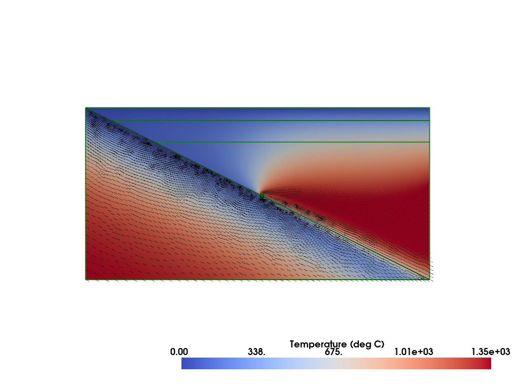
As well as visualizing the solutions we can see what effect varying the coupling depth has on the global diagnostics from the benchmark.
# print the varying coupling depth output
print('')
print('{:<12} {:<12} {:<12} {:<12} {:<12} {:<12}'.format('d_c', 'T_ndof', 'T_{200,-100}', 'Tbar_s', 'Tbar_w', 'Vrmsw'))
for dc, diag in zip(coupling_depths, diagnostics):
    print('{:<12.4g} {:<12d} {:<12.4f} {:<12.4f} {:<12.4f} {:<12.4f}'.format(dc, *diag.values()))
d_c          T_ndof       T_{200,-100} Tbar_s       Tbar_w       Vrmsw
60           15174        681.2323     518.8714     1135.5150    54.9085
80           15218        682.7046     571.7531     934.5601     40.9717
100          15214        368.7376     362.5595     571.7945     23.6382
Note the dramatic drop in temperature at (200, -100), T_{200,-100}, once the coupling depth reaches 100km.
In the next notebook we will try more realistic geometries.