Subduction Zone Benchmark#
Parallel Scaling#
In the previous notebook we tested that the error in our implementation of a steady-state thermal convection problem in two-dimensions converged towards the published benchmark value as the resolution scale (resscale) decreased (the number of elements increased). We also wish to test for parallel scaling of this problem, assessing if the simulation wall time decreases as the number of processors used to solve it is increases.
Here we perform strong scaling tests on our functions solve_benchmark_case1 and solve_benchmark_case2 from the previous notebook.
Preamble#
We start by loading all the modules we will require.
import sys, os
basedir = ''
if "__file__" in globals(): basedir = os.path.dirname(__file__)
path = os.path.join(basedir, os.path.pardir, os.path.pardir, 'python')
sys.path.insert(0, path)
import fenics_sz.utils.ipp
import matplotlib.pyplot as pl
import matplotlib.ticker as ticker
import numpy as np
import pathlib, json
output_folder = pathlib.Path(os.path.join(basedir, "output"))
output_folder.mkdir(exist_ok=True, parents=True)
Implementation#
We perform the strong parallel scaling test using a utility function (from python/utils/ipp.py) that loops over a list of the number of processors calling our function for a given resolution scale, rescale. It runs our function solve_benchmark_case1 a specified number of times and evaluates and returns the time taken for each of a number of requested steps.
# the list of the number of processors we will use
nprocs_scale = [1, 2, 4]

# resolution scale factor (equivalent to minimum element size)
resscale_scale = 2

# perform the calculation a set number of times
number = 1

# We are interested in the time to create the mesh,
# declare the functions, assemble the problem and solve it.
# From our implementation in `solve_poisson_2d` it is also
# possible to request the time to declare the Dirichlet and
# Neumann boundary conditions and the forms.
steps = [
          'Assemble Temperature', 'Assemble Stokes',
          'Solve Temperature', 'Solve Stokes'
         ]
Case 1 - Direct#
We start by running benchmark case 1 - isoviscous - and will compare direct and iterative solver strategies.
# declare a dictionary to store the times each step takes
maxtimes_1 = {}
maxtimes_mumps_1 = {}
extradiag_1 = {}
petsc_options_s = {'ksp_type':'preonly',
                   'pc_type':'lu',
                   'pc_factor_mat_solver_type' : 'mumps',
                   'mat_mumps_icntl_4': 2,
                  }

def extra_parallel_diagnostics(sz):
    diag = dict()
    bs = sz.Vslab_v.dofmap.index_map_bs # assumed the same
    diag['T_ndofs']   = sz.V_T.dofmap.index_map.size_local
    diag['T_nghosts'] = sz.V_T.dofmap.index_map.num_ghosts
    diag['v_wedge_ndofs']   = None
    diag['v_wedge_nghosts'] = None
    diag['p_wedge_ndofs']   = None
    diag['p_wedge_nghosts'] = None
    diag['v_slab_ndofs']    = None
    diag['v_slab_nghosts']  = None
    diag['p_slab_ndofs']    = None
    diag['p_slab_nghosts']  = None
    if sz.wedge_rank:
        diag['v_wedge_ndofs']   = sz.Vwedge_v.dofmap.index_map.size_local*bs
        diag['v_wedge_nghosts'] = sz.Vwedge_v.dofmap.index_map.num_ghosts*bs
        diag['p_wedge_ndofs']   = sz.Vwedge_p.dofmap.index_map.size_local
        diag['p_wedge_nghosts'] = sz.Vwedge_p.dofmap.index_map.num_ghosts
    if sz.slab_rank:
        diag['v_slab_ndofs']    = sz.Vslab_v.dofmap.index_map.size_local*bs
        diag['v_slab_nghosts']  = sz.Vslab_v.dofmap.index_map.num_ghosts*bs
        diag['p_slab_ndofs']    = sz.Vslab_p.dofmap.index_map.size_local
        diag['p_slab_nghosts']  = sz.Vslab_p.dofmap.index_map.num_ghosts
    return diag

maxtimes_1['Direct Stokes'], maxtimes_mumps_1['Direct Stokes'], extradiag_1['Direct Stokes'] = \
                   fenics_sz.utils.ipp.profile_parallel(nprocs_scale, steps, path,
                                                        'fenics_sz.sz_problems.sz_benchmark', 'solve_benchmark_case1',
                                                        resscale_scale, number=number, include_mumps_times=True,
                                                        extra_diagnostics_func=extra_parallel_diagnostics,
                                                        petsc_options_s=petsc_options_s,
                                                        output_filename=output_folder / 'sz_benchmark_scaling_direct_1.png')
=========================
                      1           2           4
Assemble Temperature  0.03        0.02        0.02
Assemble Stokes       0.07        0.04        0.05
Solve Temperature     0.23        0.23        0.26
Solve Stokes          0.54        0.37        0.43
=========================
MUMPS analysis        0.3274      0.226       0.3024
MUMPS factorization   0.1564      0.11        0.1
MUMPS solve           0.0139      0.0091      0.0079
=========================
T_ndofs_max           32749       24740       8331
T_ndofs_min           32749       8009        8000
T_ndofs_sum           32749       32749       32749
T_ndofs_avg           32749       16374.5     8187.25
T_nghosts_max         0           191         200
T_nghosts_min         0           184         87
T_nghosts_sum         0           375         585
T_nghosts_avg         0           187.5       146.25
v_wedge_ndofs_max     32408       32408       13380
v_wedge_ndofs_min     32408       32408       6192
v_wedge_ndofs_sum     32408       32408       32408
v_wedge_ndofs_avg     32408       16204       8102
v_wedge_nghosts_max   0           0           146
v_wedge_nghosts_min   0           0           60
v_wedge_nghosts_sum   0           0           296
v_wedge_nghosts_avg   0           0           74
p_wedge_ndofs_max     4128        4128        1685
p_wedge_ndofs_min     4128        4128        806
p_wedge_ndofs_sum     4128        4128        4128
p_wedge_ndofs_avg     4128        2064        1032
p_wedge_nghosts_max   0           0           45
p_wedge_nghosts_min   0           0           11
p_wedge_nghosts_sum   0           0           75
p_wedge_nghosts_avg   0           0           18.75
v_slab_ndofs_max      16400       16400       16400
v_slab_ndofs_min      16400       16400       16400
v_slab_ndofs_sum      16400       16400       16400
v_slab_ndofs_avg      16400       8200        4100
v_slab_nghosts_max    0           0           0
v_slab_nghosts_min    0           0           0
v_slab_nghosts_sum    0           0           0
v_slab_nghosts_avg    0           0           0
p_slab_ndofs_max      2115        2115        2115
p_slab_ndofs_min      2115        2115        2115
p_slab_ndofs_sum      2115        2115        2115
p_slab_ndofs_avg      2115        1057.5      528.75
p_slab_nghosts_max    0           0           0
p_slab_nghosts_min    0           0           0
p_slab_nghosts_sum    0           0           0
p_slab_nghosts_avg    0           0           0
=========================
***********  profiling figure in output/sz_benchmark_scaling_direct_1.png
# # a case using not partitioning by region for comparison
# petsc_options_s = {'ksp_type':'preonly',
#                    'pc_type':'lu',
#                    'pc_factor_mat_solver_type' : 'mumps',
#                    'mat_mumps_icntl_4': 2,
#                   }

# maxtimes_1['Direct Stokes nosplit'], maxtimes_mumps_1['Direct Stokes nosplit'], extradiag_1['Direct Stokes nosplit']  = \
#                     fenics_sz.utils.ipp.profile_parallel(nprocs_scale, steps, path,
#                                                          'fenics_sz.sz_problems.sz_benchmark', 'solve_benchmark_case1',
#                                                          resscale_scale, number=number, include_mumps_times=True,
#                                                          extra_diagnostics_func=extra_parallel_diagnostics,
#                                                          petsc_options_s=petsc_options_s, partition_by_region=False,
#                                                          output_filename=output_folder / 'sz_benchmark_nosplit_scaling_direct_1.png')
The behavior of the scaling test will strongly depend on the computational resources available on the machine where this notebook is run. In particular when the website is generated it has to run as quickly as possible on github, hence we limit our requested numbers of processors, size of the problem (resscale) and number of calculations to average over (number) in the default setup of this notebook.
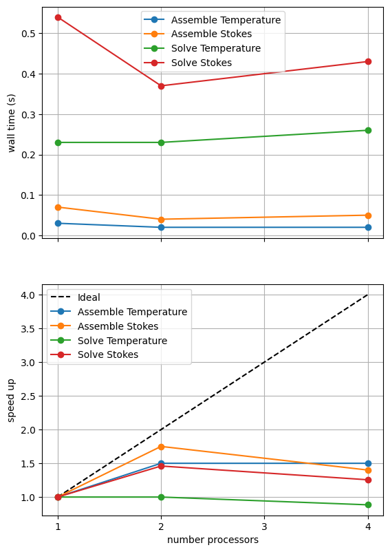
For comparison we provide the output of this notebook using resscale = 0.5 and number = 10 in Figure 3.4.1 generated on a dedicated machine with a local conda installation of the software.
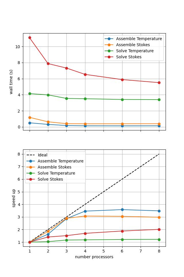
Figure 3.4.1 Scaling results for a direct solver with resscale = 0.5 averaged over number = 10 calculations using a local conda installation of the software on a dedicated machine.
We can see in Figure 3.4.1 that assembly scales well up to four processes at this resolution. As in previous scaling tests on steady state problems we see that the direct solves do not scale but that the Stokes solves (in the slab and wedge) are more expensive than the (global) temperature solve.
We also need to test that we are still converging to the benchmark solutions in parallel.
# the list of the number of processors to test the convergence on
nprocs_conv = [1, 4,]

# List of resolutions to try
resscales_conv = [2,]
diagnostics = []
for resscalel in resscales_conv:
    diagnostics.append(fenics_sz.utils.ipp.run_parallel(nprocs_conv, path,
                                           'fenics_sz.sz_problems.sz_benchmark',
                                           'benchmark_case1_diagnostics',
                                           resscalel))

print('')
print('{:<12} {:<12} {:<12} {:<12} {:<12} {:<12} {:<12}'.format('nprocs', 'resscale', 'T_ndof', 'T_{200,-100}', 'Tbar_s', 'Tbar_w', 'Vrmsw'))
for resscalel, diag_all in zip(resscales_conv, diagnostics):
    for i, nproc in enumerate(nprocs_conv):
        print('{:<12d} {:<12.4g} {:<12d} {:<12.4f} {:<12.4f} {:<12.4f} {:<12.4f}'.format(nproc, resscalel, *diag_all[i].values()))
         # check error (compared to the serial case) is less than 0.1%
        if i > 0:
            for k, v in diag_all[i].items():
                assert(abs(v - diag_all[0][k])/abs(diag_all[0][k]) < 1.e-3)
nprocs       resscale     T_ndof       T_{200,-100} Tbar_s       Tbar_w       Vrmsw
1            2            32749        516.9332     451.6764     926.2604     34.6379
4            2            32749        516.9332     451.6764     926.2604     34.6379
Case 1 - Iterative#
We can try to improve the scaling of the Stokes solution steps by using an iterative solver.
petsc_options_s = {'ksp_type':'minres',
                   'ksp_rtol' : 5.e-9,
                   'pc_type':'fieldsplit',
                   'pc_fieldsplit_type': 'additive',
                   'fieldsplit_v_ksp_type':'preonly',
                   'fieldsplit_v_pc_type':'gamg',
                   'pc_gamg_threshold_scale' : 1.0,
                   'pc_gamg_threshold' : 0.01,
                   'pc_gamg_coarse_eq_limit' : 800,
                   'fieldsplit_p_ksp_type':'preonly',
                   'fieldsplit_p_pc_type':'jacobi'}

maxtimes_1['Iterative Stokes'], _, _ = fenics_sz.utils.ipp.profile_parallel(nprocs_scale, steps, path,
                                                            'fenics_sz.sz_problems.sz_benchmark', 'solve_benchmark_case1',
                                                            resscale_scale, petsc_options_s=petsc_options_s, number=number,
                                                            output_filename=output_folder / 'sz_benchmark_scaling_iterative_1.png')
=========================
                      1           2           4
Assemble Temperature  0.03        0.03        0.02
Assemble Stokes       0.09        0.06        0.06
Solve Temperature     0.23        0.23        0.27
Solve Stokes          0.84        0.61        0.5
=========================
*********** profiling figure in output/sz_benchmark_scaling_iterative_1.png
If sufficient computational resources are available when running this notebook (unlikely during website generation) this should show that the iterative method scales better than the direct method but has a much higher absolute cost (wall time).
For reference we provide the output of this notebook using resscale = 0.5 and number = 10 in Figure 3.4.2 generated on a dedicated machine with a local conda installation of the software.
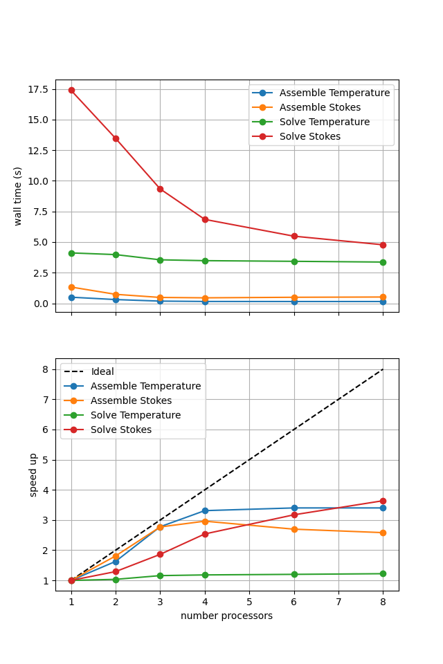
Figure 3.4.2 Scaling results for a direct solver with resscale = 0.5 averaged over number = 10 calculations using a local conda installation of the software on a dedicated machine.
Here we can see the improved scaling (for the Stokes solve, the temperature is still using a direct method) but increased cost.
We also test if the iterative method is converging to the benchmark solution below.
diagnostics = []
for resscalel in resscales_conv:
    diagnostics.append(fenics_sz.utils.ipp.run_parallel(nprocs_conv, path,
                                           'fenics_sz.sz_problems.sz_benchmark',
                                           'benchmark_case1_diagnostics',
                                           resscalel, petsc_options_s=petsc_options_s))

print('')
print('{:<12} {:<12} {:<12} {:<12} {:<12} {:<12} {:<12}'.format('nprocs', 'resscale', 'T_ndof', 'T_{200,-100}', 'Tbar_s', 'Tbar_w', 'Vrmsw'))
for resscalel, diag_all in zip(resscales_conv, diagnostics):
    for i, nproc in enumerate(nprocs_conv):
        print('{:<12d} {:<12.4g} {:<12d} {:<12.4f} {:<12.4f} {:<12.4f} {:<12.4f}'.format(nproc, resscalel, *diag_all[i].values()))
         # check error (compared to the serial case) is less than 0.1%
        if i > 0:
            for k, v in diag_all[i].items():
                assert(abs(v - diag_all[0][k])/abs(diag_all[0][k]) < 1.e-3)
nprocs       resscale     T_ndof       T_{200,-100} Tbar_s       Tbar_w       Vrmsw
1            2            32749        516.9332     451.6764     926.2605     34.6379
4            2            32749        516.9332     451.6764     926.2605     34.6379
Comparison#
We can more easily compare the different solution method directly by plotting their walltimes for assembly and solution.
# choose which steps to compare
compare_steps = ['Assemble Stokes', 'Solve Stokes']

# set up a figure for plotting
fig, axs = pl.subplots(nrows=len(compare_steps), figsize=[6.4,4.8*len(compare_steps)], sharex=True)
if len(compare_steps) == 1: axs = [axs]
for i, step in enumerate(compare_steps):
    s = steps.index(step)
    for name, lmaxtimes in maxtimes_1.items():
        axs[i].plot(nprocs_scale, [t[s] for t in lmaxtimes], 'o-', label=name)
    axs[i].xaxis.set_major_locator(ticker.MaxNLocator(integer=True))
    axs[i].set_title(step)
    axs[i].legend()
    axs[i].set_ylabel('wall time (s)')
    axs[i].grid()
axs[-1].set_xlabel('number processors')
# save the figure
fig.savefig(output_folder / 'sz_benchmark_scaling_comparison_1.png')
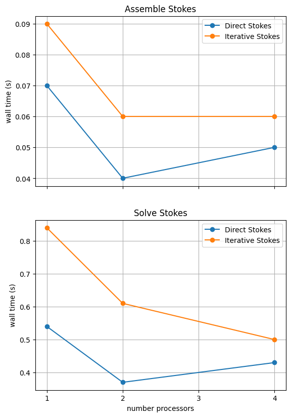
With sufficient computational resources we will see that both methods have approximately the same assembly costs but the iterative methods solution wall time costs only become competitive above approximately four processes (for resscale = 0.5) at which point the assembly scaling has stalled anyway.
For reference we provide the output of this notebook using resscale = 0.5 and number = 10 in Figure 3.4.3 generated on a dedicated machine with a local conda installation of the software.
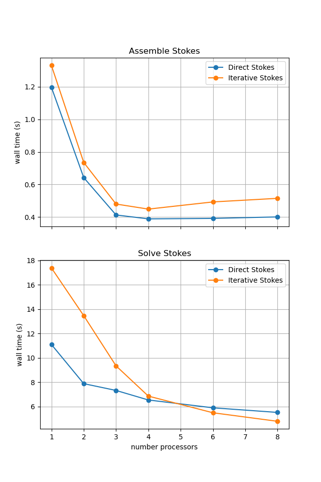
Figure 3.4.3 Scaling results for a direct solver with resscale = 0.5 averaged over number = 10 calculations using a local conda installation of the software on a dedicated machine.
Save the output for use later.
with open(output_folder/"maxtimes_1.json", "w") as f:
    json.dump(maxtimes_1, f, indent=4)
with open(output_folder/"maxtimes_mumps_1.json", "w") as f:
    json.dump(maxtimes_mumps_1, f, indent=4)
with open(output_folder/"extradiag_1.json", "w") as f:
    json.dump(extradiag_1, f, indent=4)
Case 2 - Direct#
Time constraints mean we do not run case 2 - temperature and strain-rate dependent rheology - but we do present some previously run results below.
Uncommenting the cells below will allow the direct solution strategy to be tested interactively.
# declare a dictionary to store the times each step takes
maxtimes_2 = {}
maxtimes_mumps_2 = {}
extradiag_2 = {}

# note that the iterative solver requires sufficient resolution to converge
# in the non-linear case so we decrease the resscale for these cases
resscale_scale_2 = 0.5
resscales_conv_2 = [0.5,]
# petsc_options_s = {'ksp_type':'preonly',
#                    'pc_type':'lu',
#                    'pc_factor_mat_solver_type' : 'mumps',
#                    'mat_mumps_icntl_4': 2,
#                   }

# maxtimes_2['Direct Stokes'], maxtimes_mumps_2['Direct Stokes'], extradiag_2['Direct Stokes'] = \
#                     fenics_sz.utils.ipp.profile_parallel(nprocs_scale, steps, path,
#                                                          'fenics_sz.sz_problems.sz_benchmark', 'solve_benchmark_case2',
#                                                         resscale_scale_2, number=number, include_mumps_times=True,
#                                                          extra_diagnostics_func=extra_parallel_diagnostics,
#                                                          petsc_options_s=petsc_options_s,
#                                                         output_filename=output_folder / 'sz_benchmark_scaling_direct_2.png')
# # # a case using not partitioning by region for comparison
# # petsc_options_s = {'ksp_type':'preonly',
# #                    'pc_type':'lu',
# #                    'pc_factor_mat_solver_type' : 'mumps',
# #                    'mat_mumps_icntl_4': 2,
# #                   }

# # maxtimes_2['Direct Stokes nosplit'], maxtimes_mumps_2['Direct Stokes nosplit'], extradiag_2['Direct Stokes nosplit'] = \
# #                     fenics_sz.utils.ipp.profile_parallel(nprocs_scale, steps, path,
# #                                                          'fenics_sz.sz_problems.sz_benchmark', 'solve_benchmark_case2',
# #                                                         resscale_scale_2, number=number, include_mumps_times=True,
# #                                                          extra_diagnostics_func=extra_parallel_diagnostics,
# #                                                         petsc_options_s=petsc_options_s, partition_by_region=False,
# #                                                         output_filename=output_folder / 'sz_benchmark_nosplit_scaling_direct_2.png')
As before, the behavior of the scaling test will strongly depend on the computational resources available on the machine where this notebook is run.
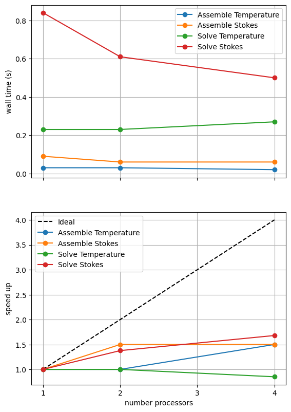
For comparison we provide the output of this notebook using resscale = 0.5 and number = 10 in Figure 3.4.4 generated on a dedicated machine with a local conda installation of the software.
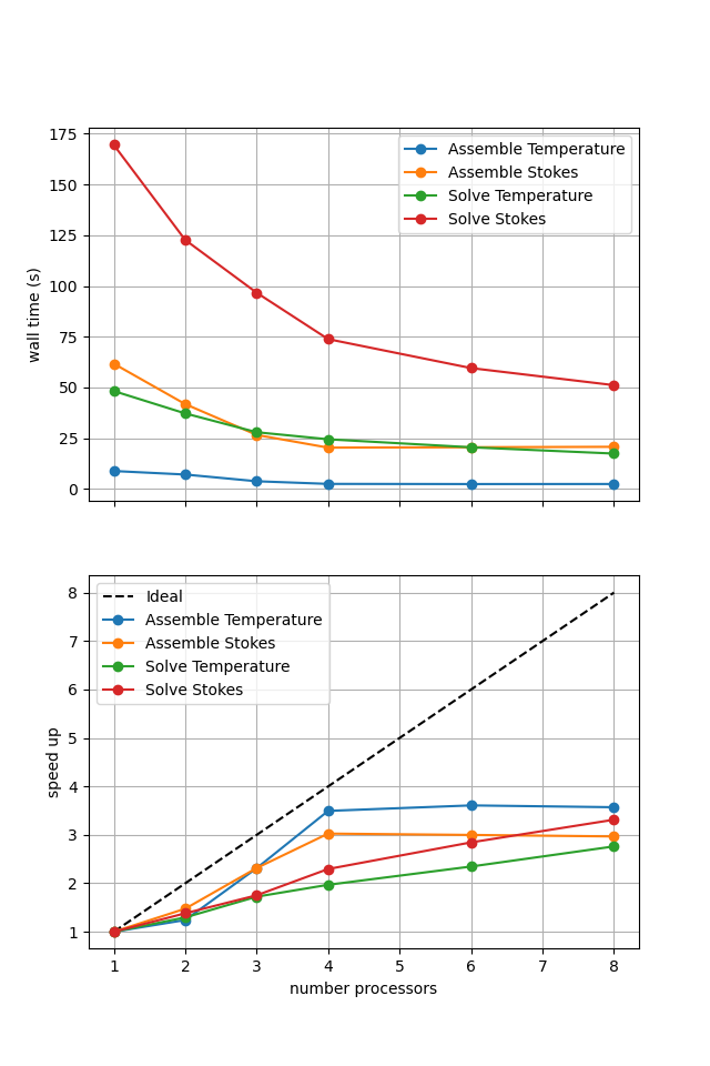
Figure 3.4.4 Scaling results for a direct solver with resscale = 0.5 averaged over number = 10 calculations using a local conda installation of the software on a dedicated machine.
We can see in Figure 3.4.4 that assembly scales well. The improved scaling behavior of the solves seen in non-linear Blankenbach convection case is seen again. This is likely because case 2 takes multiple non-linear iterations, caching the direct solver’s initial analysis step between iterations and improving the scaling relative to the linear case 1.
We can also test that we are still converging to the benchmark solutions in parallel.
# diagnostics = []
# for resscalel in resscales_conv_2:
#     diagnostics.append(fenics_sz.utils.ipp.run_parallel(nprocs_conv, path,
#                                            'fenics_sz.sz_problems.sz_benchmark',
#                                            'benchmark_case2_diagnostics',
#                                            resscalel))

# print('')
# print('{:<12} {:<12} {:<12} {:<12} {:<12} {:<12} {:<12}'.format('nprocs', 'resscale', 'T_ndof', 'T_{200,-100}', 'Tbar_s', 'Tbar_w', 'Vrmsw'))
# for resscalel, diag_all in zip(resscales_conv_2, diagnostics):
#     for i, nproc in enumerate(nprocs_conv):
#         print('{:<12d} {:<12.4g} {:<12d} {:<12.4f} {:<12.4f} {:<12.4f} {:<12.4f}'.format(nproc, resscalel, *diag_all[i].values()))
#          # check error (compared to the serial case) is less than 0.1%
#         if i > 0:
#             for k, v in diag_all[i].items():
#                 assert(abs(v - diag_all[0][k])/abs(diag_all[0][k]) < 1.e-3)
Case 2 - Iterative#
Time constraints mean we do not run case 2 - temperature and strain-rate dependent rheology - but do present some previously run results below.
Uncommenting the cells below will allow the iterative solution strategy to be tested interactively.
# petsc_options_s = {'ksp_type':'minres',
#                    'ksp_rtol' : 5.e-9,
#                    'pc_type':'fieldsplit',
#                    'pc_fieldsplit_type': 'additive',
#                    'fieldsplit_v_ksp_type':'preonly',
#                    'fieldsplit_v_pc_type':'gamg',
#                    'pc_gamg_threshold_scale' : 1.0,
#                    'pc_gamg_threshold' : 0.01,
#                    'pc_gamg_coarse_eq_limit' : 800,
#                    'fieldsplit_p_ksp_type':'preonly',
#                    'fieldsplit_p_pc_type':'jacobi'}

# maxtimes_2['Iterative Stokes'], _, _ = fenics_sz.utils.ipp.profile_parallel(nprocs_scale, steps, path,
#                                                             'fenics_sz.sz_problems.sz_benchmark', 'solve_benchmark_case2',
#                                                             resscale_scale_2, petsc_options_s=petsc_options_s, number=number,
#                                                             output_filename=output_folder / 'sz_benchmark_scaling_iterative_2.png')
If sufficient computational resources are available when running this cell interactively this should show that the iterative method scales better than the direct method but has a much higher absolute cost (wall time).
For reference we provide the output of this notebook using resscale = 0.5 and number = 10 in Figure 3.4.5 generated on a dedicated machine with a local conda installation of the software.
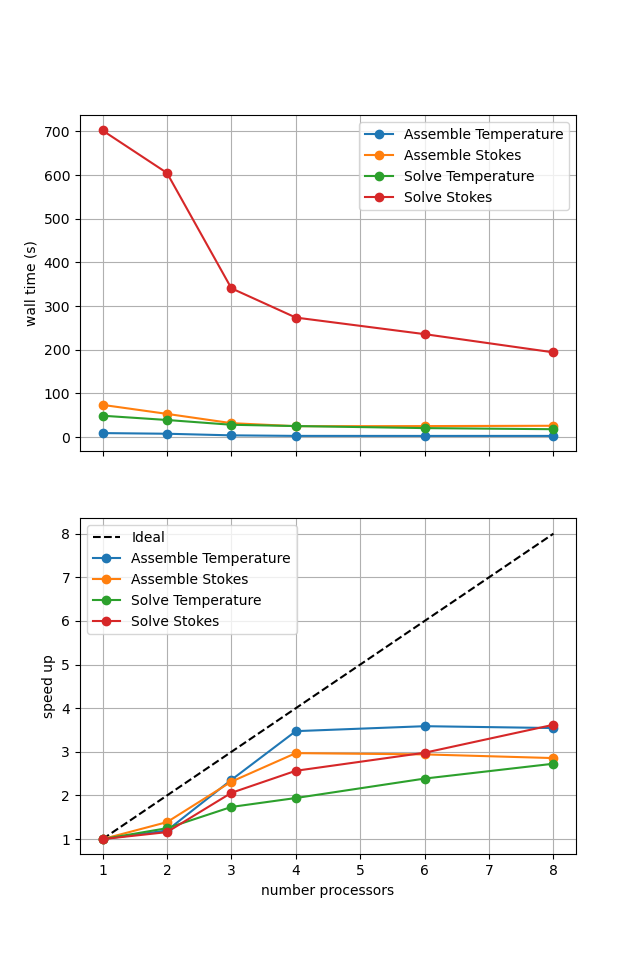
Figure 3.4.5 Scaling results for a direct solver with resscale = 0.5 averaged over number = 10 calculations using a local conda installation of the software on a dedicated machine.
Here we can see the improved scaling (for the Stokes solve, the temperature is still using a direct method) but hugely increased cost. This increase is even more significant here as the non-linearity in case 2 compared to 1 has increased the number of nonlinear iterations taken and the iterative method does not take advantage of the analysis caching employed by the direct solver strategy.
We can also test if the iterative method is converging to the benchmark solution by uncommenting the cells below.
# diagnostics = []
# for resscalel in resscales_conv_2:
#     diagnostics.append(fenics_sz.utils.ipp.run_parallel(nprocs_conv, path,
#                                            'fenics_sz.sz_problems.sz_benchmark',
#                                            'benchmark_case2_diagnostics',
#                                            resscalel, petsc_options_s=petsc_options_s))

# print('')
# print('{:<12} {:<12} {:<12} {:<12} {:<12} {:<12} {:<12}'.format('nprocs', 'resscale', 'T_ndof', 'T_{200,-100}', 'Tbar_s', 'Tbar_w', 'Vrmsw'))
# for resscalel, diag_all in zip(resscales_conv_2, diagnostics):
#     for i, nproc in enumerate(nprocs_conv):
#         print('{:<12d} {:<12.4g} {:<12d} {:<12.4f} {:<12.4f} {:<12.4f} {:<12.4f}'.format(nproc, resscalel, *diag_all[i].values()))
#          # check error (compared to the serial case) is less than 0.1%
#         if i > 0:
#             for k, v in diag_all[i].items():
#                 assert(abs(v - diag_all[0][k])/abs(diag_all[0][k]) < 1.e-3)
Case 2 - Comparison#
Time constraints mean we do not run case 2 - temperature and strain-rate dependent rheology - but do present some previously run results below.
Uncommenting the cells below will allow the solution strategies to be compared interactively.
# # choose which steps to compare
# compare_steps = ['Assemble Stokes', 'Solve Stokes']

# # set up a figure for plotting
# fig, axs = pl.subplots(nrows=len(compare_steps), figsize=[6.4,4.8*len(compare_steps)], sharex=True)
# if len(compare_steps) == 1: axs = [axs]
# for i, step in enumerate(compare_steps):
#     s = steps.index(step)
#     for name, lmaxtimes in maxtimes_2.items():
#         axs[i].plot(nprocs_scale, [t[s] for t in lmaxtimes], 'o-', label=name)
#     axs[i].xaxis.set_major_locator(ticker.MaxNLocator(integer=True))
#     axs[i].set_title(step)
#     axs[i].legend()
#     axs[i].set_ylabel('wall time (s)')
#     axs[i].grid()
# axs[-1].set_xlabel('number processors')
# # save the figure
# fig.savefig(output_folder / 'sz_benchmark_scaling_comparison_2.png')
If running interactively with sufficient computational resources we will see that both methods have approximately the same assembly costs but the iterative methods wall time costs are substantially higher and never become competitive despite scaling better at higher number of processors.
For reference we provide the output of this notebook using resscale = 0.5 and number = 10 in Figure 3.4.6 generated on a dedicated machine using a local conda installation of the software.
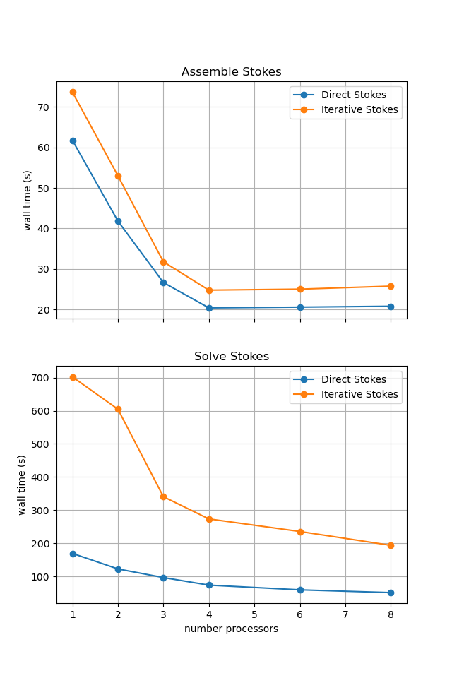
Figure 3.4.6 Scaling results for a direct solver with resscale = 0.5 averaged over number = 10 calculations using a local conda installation of the software on a dedicated machine.
Save the output for use later.
with open(output_folder/"maxtimes_2.json", "w") as f:
    json.dump(maxtimes_2, f, indent=4)
with open(output_folder/"maxtimes_mumps_2.json", "w") as f:
    json.dump(maxtimes_mumps_2, f, indent=4)
with open(output_folder/"extradiag_2.json", "w") as f:
    json.dump(extradiag_2, f, indent=4)
In the next section we will apply what we have learned here to the global suite of subduction zone thermal solvers. First however we implement a time-dependent subduction problem.