Time-Dependent Subduction Zone Setup#
Implementation#
Recalling our implementation strategy we are following a similar workflow to that seen in the background examples.
we will describe the subduction zone geometry and tesselate it into non-overlapping triangles to create a mesh
we will declare function spaces for the temperature, wedge velocity and pressure, and slab velocity and pressure
using these function space we will declare trial and test functions
we will define Dirichlet boundary conditions at the boundaries as described in the introduction
we will describe discrete weak forms for temperature and each of the coupled velocity-pressure systems that will be used to assemble the matrices (and vectors) to be solved
we will set up matrices and solvers for the discrete systems of equations
we will solve the matrix problems
For the time-dependent cases we have now implemented all but the rheology specific final step of solving the coupled velocity-pressure-temperature problem. In this notebook we do this for the case of a dislocation creep rheology, deriving a new TDDislSubductionProblem class from the TDSubductionProblem class we implemented in notebooks/03_sz_problems/3.5a_sz_tdep_problem.ipynb.
Preamble#
Let’s start by adding the path to the modules in the python folder to the system path (so we can find the our custom modules).
import sys, os
basedir = ''
if "__file__" in globals(): basedir = os.path.dirname(__file__)
sys.path.insert(0, os.path.join(basedir, os.path.pardir, os.path.pardir, 'python'))
Let’s also load the module generated by the previous notebooks to get access to the parameters and functions defined there.
from fenics_sz.sz_problems.sz_params import default_params, allsz_params
from fenics_sz.sz_problems.sz_slab import create_slab
from fenics_sz.sz_problems.sz_geometry import create_sz_geometry
from fenics_sz.sz_problems.sz_problem import StokesSolverNest, TemperatureSolver
from fenics_sz.sz_problems.sz_tdep_problem import TDSubductionProblem
Then let’s load all the required modules at the beginning.
import fenics_sz.geometry as geo
import fenics_sz.utils
from mpi4py import MPI
import dolfinx as df
import dolfinx.fem.petsc
from petsc4py import PETSc
import numpy as np
import scipy as sp
import ufl
import basix.ufl as bu
import matplotlib.pyplot as pl
import copy
import pyvista as pv
import pathlib
output_folder = pathlib.Path(os.path.join(basedir, "output"))
output_folder.mkdir(exist_ok=True, parents=True)
TDDislSubductionProblem class#
We build on the TDSubductionProblem class implemented in notebooks/03_sz_problems/3.5a_sz_tdep_problem.ipynb, deriving a TDDislSubductionProblem class that implements and solves the equations for a time-dependent dislocation creep case.
7. Solution#
Solving for the thermal state of the subduction zone is more complicated when using a dislocation creep viscosity than in the isoviscous rheology case due to the non-linearities introduced by having the viscosity depend on both temperature and velocity (through the strain rate). These mean that we not only need a time-loop but also must iterate between the velocity and temperature solutions until a (hopefully) converged solution is achieved at each time-step. Due to the split nature of our submeshes we do this using a Picard or fixed-point iteration.
At each timestep the iteration convergence is tested by calculating the residual of each subproblem and ensuring that their norm is small either in a relative (to the initial residual that timestep, rtol) or absolute (atol) sense. To prevent a runaway non-converging computation we place a maximum cap on the number of iterations (maxits) that the iteration may take each timestep. The number of iterations taken is generally much lower in a time-dependent case because the initial guess each timestep (the solution from the previous timestep) is much closer to the converged solution. This iteration every timestep can take some time, particularly at high resolutions (low resscales).
The timestep size is controlled by dt, which should be chosen to be small enough, depending on the implicitness parameter, theta, to ensure a stable solution. The size of dt will also influence the time it takes to reach the final solution, at time tf.
To evaluate the residual norm we implement the function calculate_residual before using it in the solve function.
class TDDislSubductionProblem(TDSubductionProblem):
    def calculate_residual(self, rw, rs, rT):
        """
        Given forms for the vpw, vps and T residuals,
        return the total residual of the problem.

        Arguments:
          * rw - residual form for the wedge velocity and pressure
          * rs - residual form for the slab velocity and pressure
          * rT - residual form for the temperature

        Returns:
          * r  - 2-norm of the combined residual
        """
        # because some of our forms are defined on different MPI comms
        # we need to calculate a squared 2-norm locally and use the global
        # comm to reduce it
        def calc_r_norm_sq(r, bcs, this_rank=True):
            r_norm_sq = 0.0
            if this_rank:
                r_vec = df.fem.petsc.assemble_vector_nest(r)
                # update the ghost values
                for r_vec_sub in r_vec.getNestSubVecs():
                    r_vec_sub.ghostUpdate(addv=PETSc.InsertMode.ADD, mode=PETSc.ScatterMode.REVERSE)
                # set bcs
                bcs_by_block = df.fem.bcs_by_block(df.fem.extract_function_spaces(r), bcs)
                df.fem.petsc.set_bc_nest(r_vec, bcs_by_block, alpha=0.0)
                r_arr = r_vec.getArray()
                r_norm_sq = np.inner(r_arr, r_arr)
            return r_norm_sq
        with df.common.Timer("Assemble Stokes"):
            r_norm_sq  = calc_r_norm_sq(rw, self.bcs_vw, self.wedge_rank)
            r_norm_sq += calc_r_norm_sq(rs, self.bcs_vs, self.slab_rank)
        self.comm.barrier()
        with df.common.Timer("Assemble Temperature"):
            r_norm_sq += calc_r_norm_sq(rT, self.bcs_T)
        r = self.comm.allreduce(r_norm_sq, op=MPI.SUM)**0.5
        return r

    def solve(self, tf, dt, theta=0.5, rtol=5.e-6, atol=5.e-9, maxits=50, verbosity=2,
              petsc_options_s=None, petsc_options_T=None,
              plotter=None):
        """
        Solve the coupled temperature-velocity-pressure problem assuming a dislocation creep rheology with time dependency

        Arguments:
          * tf - final time  (in Myr)
          * dt - the timestep (in Myr)

        Keyword Arguments:
          * theta         - theta parameter for timestepping (0 <= theta <= 1, defaults to theta=0.5)
          * rtol          - nonlinear iteration relative tolerance
          * atol          - nonlinear iteration absolute tolerance
          * maxits        - maximum number of nonlinear iterations
          * verbosity     - level of verbosity (<1=silent, >0=basic, >1=timestep, >2=nonlinear convergence, defaults to 2)
          * petsc_options_s - a dictionary of petsc options to pass to the Stokes solver
                              (defaults to an LU direct solver using the MUMPS library)
          * petsc_options_T - a dictionary of petsc options to pass to the temperature solver
                              (defaults to an LU direct solver using the MUMPS library)
        """
        assert(theta >= 0 and theta <= 1)

        # set the timestepping options based on the arguments
        # these need to be set before calling self.temperature_forms_timedependent
        self.dt = df.fem.Constant(self.mesh, df.default_scalar_type(dt/self.t0_Myr))
        self.theta = df.fem.Constant(self.mesh, df.default_scalar_type(theta))

        # reset the initial conditions
        self.setup_boundaryconditions()

        # first solve the isoviscous problem
        self.solve_stokes_isoviscous(petsc_options=petsc_options_s)

        # retrieve the temperature forms (implemented in the parent class)
        ST, fT, rT = self.temperature_forms()
        solver_T = TemperatureSolver(ST, fT, self.bcs_T, self.T_i,
                                     petsc_options=petsc_options_T)

        # retrieve the non-linear Stokes forms for the wedge
        Ssw, fsw, rsw, Msw = self.stokes_forms(self.wedge_vw_t, self.wedge_pw_t,
                                                self.wedge_vw_a, self.wedge_pw_a,
                                                self.wedge_vw_i, self.wedge_pw_i,
                                                eta=self.etadisl(self.wedge_vw_i, self.wedge_T_i))
        # set up a solver for the wedge velocity and pressure
        solver_s_w = StokesSolverNest(Ssw, fsw, self.bcs_vw,
                                      self.wedge_vw_i, self.wedge_pw_i,
                                      M=Msw, isoviscous=False,
                                      petsc_options=petsc_options_s)

        # retrieve the non-linear Stokes forms for the slab
        Sss, fss, rss, Mss = self.stokes_forms(self.slab_vs_t, self.slab_ps_t,
                                                self.slab_vs_a, self.slab_ps_a,
                                                self.slab_vs_i, self.slab_ps_i,
                                                eta=self.etadisl(self.slab_vs_i, self.slab_T_i))
        # set up a solver for the slab velocity and pressure
        solver_s_s = StokesSolverNest(Sss, fss, self.bcs_vs,
                                      self.slab_vs_i, self.slab_ps_i,
                                      M=Mss, isoviscous=False,
                                      petsc_options=petsc_options_s)

        t = 0
        ti = 0
        tf_nd = tf/self.t0_Myr
        # time loop
        if self.comm.rank == 0 and verbosity>0:
            print("Entering timeloop with {:d} steps (dt = {:g} Myr, final time = {:g} Myr)".format(int(np.ceil(tf_nd/self.dt.value)), dt, tf,))
        # enter the time-loop
        while t < tf_nd - 1e-9:
            if self.comm.rank == 0 and verbosity>1:
                print("Step: {:>6d}, Times: {:>9g} -> {:>9g} Myr".format(ti, t*self.t0_Myr, (t+self.dt.value)*self.t0_Myr,))
            if plotter is not None:
                for mesh in plotter.meshes:
                    if self.T_i.name in mesh.point_data:
                        mesh.point_data[self.T_i.name][:] = self.T_i.x.array
                plotter.write_frame()
            # set the old solution to the new solution
            self.T_n.x.array[:] = self.T_i.x.array
            # calculate the initial residual
            r = self.calculate_residual(rsw, rss, rT)
            r0 = r
            rrel = r/r0  # 1
            if self.comm.rank == 0 and verbosity>2:
                    print("    {:<11} {:<12} {:<17}".format('Iteration','Residual','Relative Residual'))
                    print("-"*42)

            it = 0
            # enter the Picard Iteration
            if self.comm.rank == 0 and verbosity>2: print("    {:<11} {:<12.6g} {:<12.6g}".format(it, r, rrel,))
            while r > atol and rrel > rtol:
                if it > maxits: break
                # solve for temperature and interpolate it
                self.T_i = solver_T.solve()
                self.update_T_functions()

                # solve for v & p and interpolate the velocity
                if self.wedge_rank: self.wedge_vw_i, self.wedge_pw_i = solver_s_w.solve()
                if self.slab_rank:  self.slab_vs_i,  self.slab_ps_i  = solver_s_s.solve()
                self.update_v_functions()

                # wait for all ranks to catch up
                # (some may not have done anything above and
                # letting them carry on messes with profiling)
                self.comm.barrier()

                # calculate a new residual
                r = self.calculate_residual(rsw, rss, rT)
                rrel = r/r0
                # increment iterations
                it+=1
                if self.comm.rank == 0 and verbosity>2: print("    {:<11} {:<12.6g} {:<12.6g}".format(it, r, rrel,))
            # check for convergence failures
            if it > maxits:
                raise Exception("Nonlinear iteration failed to converge after {} iterations (maxits = {}), r = {} (atol = {}), rrel = {} (rtol = {}).".format(it, \
                                                                                                                                                          maxits, \
                                                                                                                                                          r, \
                                                                                                                                                          rtol, \
                                                                                                                                                          rrel, \
                                                                                                                                                          rtol,))
            # increment the timestep number
            ti+=1
            # increate time
            t+=self.dt.value
        if self.comm.rank == 0 and verbosity>0:
            print("Finished timeloop after {:d} steps (final time = {:g} Myr)".format(ti, t*self.t0_Myr,))

        # only update the pressure at the end as it is not necessary earlier
        self.update_p_functions()
Demonstration - Benchmark case 2 (time-dependent)#
resscale = 5
xs = [0.0, 140.0, 240.0, 400.0]
ys = [0.0, -70.0, -120.0, -200.0]
lc_depth = 40
uc_depth = 15
coast_distance = 0
extra_width = 0
sztype = 'continental'
io_depth = 154.0
A      = 100.0      # age of subducting slab (Myr)
qs     = 0.065      # surface heat flux (W/m^2)
Vs     = 100.0      # slab speed (mm/yr)
slab = create_slab(xs, ys, resscale, lc_depth)
geom_case2td = create_sz_geometry(slab, resscale, sztype, io_depth, extra_width,
                            coast_distance, lc_depth, uc_depth)
sz_case2td = TDDislSubductionProblem(geom_case2td, A=A, Vs=Vs, sztype=sztype, qs=qs)

sz_case2td.solve(10, 0.05, theta=0.5, rtol=1.e-3)
Entering timeloop with 200 steps (dt = 0.05 Myr, final time = 10 Myr)
Step:      0, Times:         0 ->      0.05 Myr
Step:      1, Times:      0.05 ->       0.1 Myr
Step:      2, Times:       0.1 ->      0.15 Myr
Step:      3, Times:      0.15 ->       0.2 Myr
Step:      4, Times:       0.2 ->      0.25 Myr
Step:      5, Times:      0.25 ->       0.3 Myr
Step:      6, Times:       0.3 ->      0.35 Myr
Step:      7, Times:      0.35 ->       0.4 Myr
Step:      8, Times:       0.4 ->      0.45 Myr
Step:      9, Times:      0.45 ->       0.5 Myr
Step:     10, Times:       0.5 ->      0.55 Myr
Step:     11, Times:      0.55 ->       0.6 Myr
Step:     12, Times:       0.6 ->      0.65 Myr
Step:     13, Times:      0.65 ->       0.7 Myr
Step:     14, Times:       0.7 ->      0.75 Myr
Step:     15, Times:      0.75 ->       0.8 Myr
Step:     16, Times:       0.8 ->      0.85 Myr
Step:     17, Times:      0.85 ->       0.9 Myr
Step:     18, Times:       0.9 ->      0.95 Myr
Step:     19, Times:      0.95 ->         1 Myr
Step:     20, Times:         1 ->      1.05 Myr
Step:     21, Times:      1.05 ->       1.1 Myr
Step:     22, Times:       1.1 ->      1.15 Myr
Step:     23, Times:      1.15 ->       1.2 Myr
Step:     24, Times:       1.2 ->      1.25 Myr
Step:     25, Times:      1.25 ->       1.3 Myr
Step:     26, Times:       1.3 ->      1.35 Myr
Step:     27, Times:      1.35 ->       1.4 Myr
Step:     28, Times:       1.4 ->      1.45 Myr
Step:     29, Times:      1.45 ->       1.5 Myr
Step:     30, Times:       1.5 ->      1.55 Myr
Step:     31, Times:      1.55 ->       1.6 Myr
Step:     32, Times:       1.6 ->      1.65 Myr
Step:     33, Times:      1.65 ->       1.7 Myr
Step:     34, Times:       1.7 ->      1.75 Myr
Step:     35, Times:      1.75 ->       1.8 Myr
Step:     36, Times:       1.8 ->      1.85 Myr
Step:     37, Times:      1.85 ->       1.9 Myr
Step:     38, Times:       1.9 ->      1.95 Myr
Step:     39, Times:      1.95 ->         2 Myr
Step:     40, Times:         2 ->      2.05 Myr
Step:     41, Times:      2.05 ->       2.1 Myr
Step:     42, Times:       2.1 ->      2.15 Myr
Step:     43, Times:      2.15 ->       2.2 Myr
Step:     44, Times:       2.2 ->      2.25 Myr
Step:     45, Times:      2.25 ->       2.3 Myr
Step:     46, Times:       2.3 ->      2.35 Myr
Step:     47, Times:      2.35 ->       2.4 Myr
Step:     48, Times:       2.4 ->      2.45 Myr
Step:     49, Times:      2.45 ->       2.5 Myr
Step:     50, Times:       2.5 ->      2.55 Myr
Step:     51, Times:      2.55 ->       2.6 Myr
Step:     52, Times:       2.6 ->      2.65 Myr
Step:     53, Times:      2.65 ->       2.7 Myr
Step:     54, Times:       2.7 ->      2.75 Myr
Step:     55, Times:      2.75 ->       2.8 Myr
Step:     56, Times:       2.8 ->      2.85 Myr
Step:     57, Times:      2.85 ->       2.9 Myr
Step:     58, Times:       2.9 ->      2.95 Myr
Step:     59, Times:      2.95 ->         3 Myr
Step:     60, Times:         3 ->      3.05 Myr
Step:     61, Times:      3.05 ->       3.1 Myr
Step:     62, Times:       3.1 ->      3.15 Myr
Step:     63, Times:      3.15 ->       3.2 Myr
Step:     64, Times:       3.2 ->      3.25 Myr
Step:     65, Times:      3.25 ->       3.3 Myr
Step:     66, Times:       3.3 ->      3.35 Myr
Step:     67, Times:      3.35 ->       3.4 Myr
Step:     68, Times:       3.4 ->      3.45 Myr
Step:     69, Times:      3.45 ->       3.5 Myr
Step:     70, Times:       3.5 ->      3.55 Myr
Step:     71, Times:      3.55 ->       3.6 Myr
Step:     72, Times:       3.6 ->      3.65 Myr
Step:     73, Times:      3.65 ->       3.7 Myr
Step:     74, Times:       3.7 ->      3.75 Myr
Step:     75, Times:      3.75 ->       3.8 Myr
Step:     76, Times:       3.8 ->      3.85 Myr
Step:     77, Times:      3.85 ->       3.9 Myr
Step:     78, Times:       3.9 ->      3.95 Myr
Step:     79, Times:      3.95 ->         4 Myr
Step:     80, Times:         4 ->      4.05 Myr
Step:     81, Times:      4.05 ->       4.1 Myr
Step:     82, Times:       4.1 ->      4.15 Myr
Step:     83, Times:      4.15 ->       4.2 Myr
Step:     84, Times:       4.2 ->      4.25 Myr
Step:     85, Times:      4.25 ->       4.3 Myr
Step:     86, Times:       4.3 ->      4.35 Myr
Step:     87, Times:      4.35 ->       4.4 Myr
Step:     88, Times:       4.4 ->      4.45 Myr
Step:     89, Times:      4.45 ->       4.5 Myr
Step:     90, Times:       4.5 ->      4.55 Myr
Step:     91, Times:      4.55 ->       4.6 Myr
Step:     92, Times:       4.6 ->      4.65 Myr
Step:     93, Times:      4.65 ->       4.7 Myr
Step:     94, Times:       4.7 ->      4.75 Myr
Step:     95, Times:      4.75 ->       4.8 Myr
Step:     96, Times:       4.8 ->      4.85 Myr
Step:     97, Times:      4.85 ->       4.9 Myr
Step:     98, Times:       4.9 ->      4.95 Myr
Step:     99, Times:      4.95 ->         5 Myr
Step:    100, Times:         5 ->      5.05 Myr
Step:    101, Times:      5.05 ->       5.1 Myr
Step:    102, Times:       5.1 ->      5.15 Myr
Step:    103, Times:      5.15 ->       5.2 Myr
Step:    104, Times:       5.2 ->      5.25 Myr
Step:    105, Times:      5.25 ->       5.3 Myr
Step:    106, Times:       5.3 ->      5.35 Myr
Step:    107, Times:      5.35 ->       5.4 Myr
Step:    108, Times:       5.4 ->      5.45 Myr
Step:    109, Times:      5.45 ->       5.5 Myr
Step:    110, Times:       5.5 ->      5.55 Myr
Step:    111, Times:      5.55 ->       5.6 Myr
Step:    112, Times:       5.6 ->      5.65 Myr
Step:    113, Times:      5.65 ->       5.7 Myr
Step:    114, Times:       5.7 ->      5.75 Myr
Step:    115, Times:      5.75 ->       5.8 Myr
Step:    116, Times:       5.8 ->      5.85 Myr
Step:    117, Times:      5.85 ->       5.9 Myr
Step:    118, Times:       5.9 ->      5.95 Myr
Step:    119, Times:      5.95 ->         6 Myr
Step:    120, Times:         6 ->      6.05 Myr
Step:    121, Times:      6.05 ->       6.1 Myr
Step:    122, Times:       6.1 ->      6.15 Myr
Step:    123, Times:      6.15 ->       6.2 Myr
Step:    124, Times:       6.2 ->      6.25 Myr
Step:    125, Times:      6.25 ->       6.3 Myr
Step:    126, Times:       6.3 ->      6.35 Myr
Step:    127, Times:      6.35 ->       6.4 Myr
Step:    128, Times:       6.4 ->      6.45 Myr
Step:    129, Times:      6.45 ->       6.5 Myr
Step:    130, Times:       6.5 ->      6.55 Myr
Step:    131, Times:      6.55 ->       6.6 Myr
Step:    132, Times:       6.6 ->      6.65 Myr
Step:    133, Times:      6.65 ->       6.7 Myr
Step:    134, Times:       6.7 ->      6.75 Myr
Step:    135, Times:      6.75 ->       6.8 Myr
Step:    136, Times:       6.8 ->      6.85 Myr
Step:    137, Times:      6.85 ->       6.9 Myr
Step:    138, Times:       6.9 ->      6.95 Myr
Step:    139, Times:      6.95 ->         7 Myr
Step:    140, Times:         7 ->      7.05 Myr
Step:    141, Times:      7.05 ->       7.1 Myr
Step:    142, Times:       7.1 ->      7.15 Myr
Step:    143, Times:      7.15 ->       7.2 Myr
Step:    144, Times:       7.2 ->      7.25 Myr
Step:    145, Times:      7.25 ->       7.3 Myr
Step:    146, Times:       7.3 ->      7.35 Myr
Step:    147, Times:      7.35 ->       7.4 Myr
Step:    148, Times:       7.4 ->      7.45 Myr
Step:    149, Times:      7.45 ->       7.5 Myr
Step:    150, Times:       7.5 ->      7.55 Myr
Step:    151, Times:      7.55 ->       7.6 Myr
Step:    152, Times:       7.6 ->      7.65 Myr
Step:    153, Times:      7.65 ->       7.7 Myr
Step:    154, Times:       7.7 ->      7.75 Myr
Step:    155, Times:      7.75 ->       7.8 Myr
Step:    156, Times:       7.8 ->      7.85 Myr
Step:    157, Times:      7.85 ->       7.9 Myr
Step:    158, Times:       7.9 ->      7.95 Myr
Step:    159, Times:      7.95 ->         8 Myr
Step:    160, Times:         8 ->      8.05 Myr
Step:    161, Times:      8.05 ->       8.1 Myr
Step:    162, Times:       8.1 ->      8.15 Myr
Step:    163, Times:      8.15 ->       8.2 Myr
Step:    164, Times:       8.2 ->      8.25 Myr
Step:    165, Times:      8.25 ->       8.3 Myr
Step:    166, Times:       8.3 ->      8.35 Myr
Step:    167, Times:      8.35 ->       8.4 Myr
Step:    168, Times:       8.4 ->      8.45 Myr
Step:    169, Times:      8.45 ->       8.5 Myr
Step:    170, Times:       8.5 ->      8.55 Myr
Step:    171, Times:      8.55 ->       8.6 Myr
Step:    172, Times:       8.6 ->      8.65 Myr
Step:    173, Times:      8.65 ->       8.7 Myr
Step:    174, Times:       8.7 ->      8.75 Myr
Step:    175, Times:      8.75 ->       8.8 Myr
Step:    176, Times:       8.8 ->      8.85 Myr
Step:    177, Times:      8.85 ->       8.9 Myr
Step:    178, Times:       8.9 ->      8.95 Myr
Step:    179, Times:      8.95 ->         9 Myr
Step:    180, Times:         9 ->      9.05 Myr
Step:    181, Times:      9.05 ->       9.1 Myr
Step:    182, Times:       9.1 ->      9.15 Myr
Step:    183, Times:      9.15 ->       9.2 Myr
Step:    184, Times:       9.2 ->      9.25 Myr
Step:    185, Times:      9.25 ->       9.3 Myr
Step:    186, Times:       9.3 ->      9.35 Myr
Step:    187, Times:      9.35 ->       9.4 Myr
Step:    188, Times:       9.4 ->      9.45 Myr
Step:    189, Times:      9.45 ->       9.5 Myr
Step:    190, Times:       9.5 ->      9.55 Myr
Step:    191, Times:      9.55 ->       9.6 Myr
Step:    192, Times:       9.6 ->      9.65 Myr
Step:    193, Times:      9.65 ->       9.7 Myr
Step:    194, Times:       9.7 ->      9.75 Myr
Step:    195, Times:      9.75 ->       9.8 Myr
Step:    196, Times:       9.8 ->      9.85 Myr
Step:    197, Times:      9.85 ->       9.9 Myr
Step:    198, Times:       9.9 ->      9.95 Myr
Step:    199, Times:      9.95 ->        10 Myr
Finished timeloop after 200 steps (final time = 10 Myr)
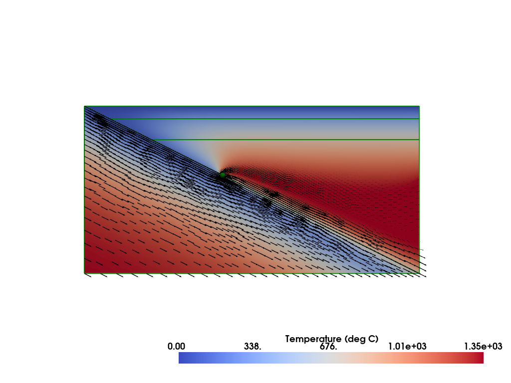
plotter_distd = fenics_sz.utils.plot.plot_scalar(sz_case2td.T_i, scale=sz_case2td.T0, gather=True, cmap='coolwarm', scalar_bar_args={'title': 'Temperature (deg C)', 'bold':True})
fenics_sz.utils.plot.plot_vector_glyphs(sz_case2td.vw_i, plotter=plotter_distd, factor=0.1, gather=True, color='k', scale=fenics_sz.utils.mps_to_mmpyr(sz_case2td.v0))
fenics_sz.utils.plot.plot_vector_glyphs(sz_case2td.vs_i, plotter=plotter_distd, factor=0.1, gather=True, color='k', scale=fenics_sz.utils.mps_to_mmpyr(sz_case2td.v0))
sz_case2td.geom.pyvistaplot(plotter=plotter_distd, color='green', width=2)
cdpt = sz_case2td.geom.slab_spline.findpoint('Slab::FullCouplingDepth')
fenics_sz.utils.plot.plot_points([[cdpt.x, cdpt.y, 0.0]], plotter=plotter_distd, render_points_as_spheres=True, point_size=10.0, color='green')
fenics_sz.utils.plot.plot_show(plotter_distd)
fenics_sz.utils.plot.plot_save(plotter_distd, output_folder / "sz_problem_case2td_solution.png")