Poisson Example 2D#
Description#
As a reminder, in this case we are seeking the approximate solution to
in a unit square, \(\Omega=[0,1]\times[0,1]\), imposing the boundary conditions
The analytical solution to this problem is \(T(x,y) = \exp\left(x+\tfrac{y}{2}\right)\).
Themes and variations#
Given that we know the exact solution to this problem is \(T(x,y) = \exp\left(x+\tfrac{y}{2}\right)\) write a python function to evaluate the error in our numerical solution.
Loop over a variety of numbers of elements,
ne, and polynomial degrees,p, and check that the numerical solution converges with an increasing number of degrees of freedom.Write an equation for the gradient of \(\tilde{T}\), describe it using UFL, solve it, and plot the solution.
Preamble#
Start by loading some required modules and functions, including solve_poisson_2d from python/fenics_sz/background/poisson_2d.py, which was automatically created at the end of notebooks/02_background/2.3b_poisson_2d.ipynb.
import sys, os
basedir = ''
if "__file__" in globals(): basedir = os.path.dirname(__file__)
sys.path.insert(0, os.path.join(basedir, os.path.pardir, os.path.pardir, 'python'))
from fenics_sz.background.poisson_2d import solve_poisson_2d
from mpi4py import MPI
import dolfinx as df
import dolfinx.fem.petsc
import numpy as np
import ufl
import fenics_sz.utils.plot
import matplotlib.pyplot as pl
import pathlib
output_folder = pathlib.Path(os.path.join(basedir, "output"))
output_folder.mkdir(exist_ok=True, parents=True)
Error analysis#
We can quantify the error in cases where the analytical solution is known by taking the L2 norm of the difference between the numerical and (known) exact solutions.
def evaluate_error(T_i):
    """
    A python function to evaluate the l2 norm of the error in
    the two dimensional Poisson problem given a known analytical
    solution.
    Parameters:
      * T_i - numerical solution
    Returns:
      * l2err - l2 norm of the error
    """
    # Define the exact solution
    x  = ufl.SpatialCoordinate(T_i.function_space.mesh)
    Te = ufl.exp(x[0] + x[1]/2.)

    # Define the error between the exact solution and the given
    # approximate solution
    l2err = df.fem.assemble_scalar(df.fem.form((T_i - Te)*(T_i - Te)*ufl.dx))
    l2err = T_i.function_space.mesh.comm.allreduce(l2err, op=MPI.SUM)**0.5

    # Return the l2 norm of the error
    return l2err
Convergence test#
Repeating the numerical experiments with increasing ne allows us to test the convergence of our approximate finite element solution to the known analytical solution. A key feature of any discretization technique is that with an increasing number of degrees of freedom (DOFs) these solutions should converge, i.e. the error in our approximation should decrease.
We implement a function, convergence_errors to loop over different polynomial orders, p, and numbers of elements, ne evaluating the error for each.
def convergence_errors(ps, nelements, petsc_options=None):
    """
    A python function to evaluate the convergence errors in a two-dimensional
    Poisson problem on a unit square domain.
    Parameters:
    * ps        - a list of polynomial orders to test
    * nelements - a list of the number of elements to test
    * petsc_options - a dictionary of petsc options to pass to the solver
                      (defaults to an LU direct solver using the MUMPS library)
    Returns:
    * errors_l2 - a list of l2 errors
    """
    errors_l2 = []
    # Loop over the polynomial orders
    for p in ps:
        # Accumulate the errors
        errors_l2_p = []
        # Loop over the resolutions
        for ne in nelements:
            # Solve the 2D Poisson problem
            T_i = solve_poisson_2d(ne, p, petsc_options=petsc_options)
            # Evaluate the error in the approximate solution
            l2error = evaluate_error(T_i)
            # Print to screen and save if on rank 0
            if MPI.COMM_WORLD.rank == 0:
                print('p={}, ne={}, l2error={}'.format(p, ne, l2error))
            errors_l2_p.append(l2error)
        if MPI.COMM_WORLD.rank == 0:
            print('*************************************************')
        errors_l2.append(errors_l2_p)

    return errors_l2
We can use this function to get the errors at a range of polynomial orders and numbers of elements.
# List of polynomial orders to try
ps = [1, 2]
# List of resolutions to try
nelements = [10, 20, 40, 80, 160]

errors_l2 = convergence_errors(ps, nelements)
p=1, ne=10, l2error=0.002714702748625412
p=1, ne=20, l2error=0.0006802808525074355
p=1, ne=40, l2error=0.00017001104597910024
p=1, ne=80, l2error=4.248277760933491e-05
p=1, ne=160, l2error=1.0618025090772703e-05
*************************************************
p=2, ne=10, l2error=2.7202419660205842e-05
p=2, ne=20, l2error=3.4296982751630815e-06
p=2, ne=40, l2error=4.3082861470124095e-07
p=2, ne=80, l2error=5.399650589936235e-08
p=2, ne=160, l2error=6.758844200882434e-09
*************************************************
Here we can see that the error is decreasing both with increasing ne and increasing p but this is clearer if we plot the errors and evaluate their order of convergence. To do this we write a python function test_plot_convergence.
def test_plot_convergence(ps, nelements, errors_l2, output_basename=None):
    """
    A python function to test and plot convergence of the given errors.
    Parameters:
    * ps              - a list of polynomial orders to test
    * nelements       - a list of the number of elements to test
    * errors_l2       - errors_l2 from convergence_errors
    * output_basename - basename for output (defaults to no output)
    Returns:
    * test_passes     - a boolean indicating if the convergence test has passed
    """

    if MPI.COMM_WORLD.rank == 0:
        # Open a figure for plotting
        fig = pl.figure()
        ax = fig.gca()

    # Keep track of whether we get the expected order of convergence
    test_passes = True

    # Loop over the polynomial orders
    for i, p in enumerate(ps):
        # Work out the order of convergence at this p
        hs = 1./np.array(nelements)/p
        # Fit a line to the convergence data
        fit = np.polyfit(np.log(hs), np.log(errors_l2[i]),1)
        # Test if the order of convergence is as expected (polynomial degree plus 1)
        test_passes = test_passes and fit[0] > p+0.9

        # Write the errors to disk
        if MPI.COMM_WORLD.rank == 0:
            if output_basename is not None:
                with open(str(output_basename) + '_p{}.csv'.format(p), 'w') as f:
                    np.savetxt(f, np.c_[nelements, hs, errors_l2[i]], delimiter=',',
                            header='nelements, hs, l2errs')

            print("order of accuracy p={}, order={:.2f}".format(p,fit[0]))

            # log-log plot of the error
            ax.loglog(hs,errors_l2[i],'o-',label='p={}, order={:.2f}'.format(p,fit[0]))


    if MPI.COMM_WORLD.rank == 0:
        # Tidy up the plot
        ax.set_xlabel(r'$h$')
        ax.set_ylabel(r'$||e||_2$')
        ax.grid()
        ax.set_title('Convergence')
        ax.legend()

        # Write convergence to disk
        if output_basename is not None:
            fig.savefig(str(output_basename) + '.pdf')

            print("***********  convergence figure in "+str(output_basename)+ ".pdf")

    # Return if we passed the test
    return test_passes
test_passes = test_plot_convergence(ps, nelements, errors_l2,
                output_basename = output_folder / '2d_poisson_convergence')

assert(test_passes)
order of accuracy p=1, order=2.00
order of accuracy p=2, order=2.99
*********** convergence figure in output/2d_poisson_convergence.pdf
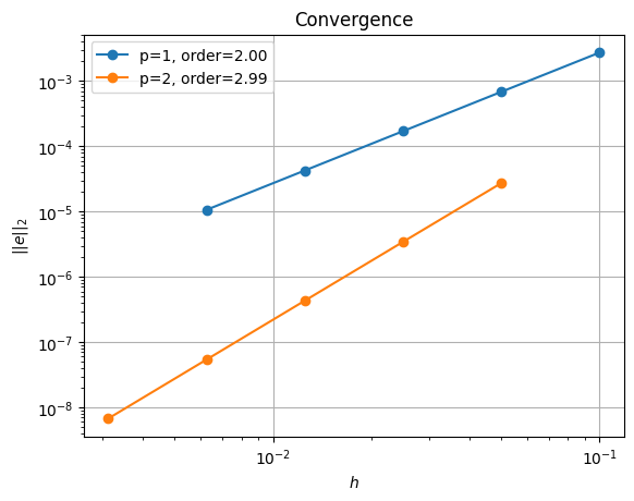
The convergence tests show that we achieve the expected orders of convergence for all polynomial degrees tested. In the next notebook we will test if this is still true when the problem is run in parallel, using multiple processors. But first we will examine how to evaluate and plot the gradient of our solution (a vector quantity).
Gradient#
To find the approximate gradient of the numerical solution \(\tilde{T}\) we seek the solution to
where \(\vec{g}\) is the gradient solution we seek in the domain \(\Omega=[0,1]\times[0,1]\). This is a projection operation and no boundary conditions are required.
We proceed as before
we solve for \(\tilde{T}\) using elements with polynomial degree
pon a mesh of \(2 \times\)ne\(\times\)netriangular elements or cellswe reuse the mesh to declare a vector function space for \(\vec{g} \approx \tilde{\vec{g}}\),
Vg, to use Lagrange polynomials of degreepgusing this function space we declare trial,
g_a, and test,g_t, functionswe define the right hand side using the gradient of \(\tilde{T}\)
we describe the discrete weak forms,
Sgandfg, that will be used to assemble the left-hand-side matrix \(\mathbf{S}_g\) and right-hand-side vector \(\mathbf{f}_g\)we solve the matrix problem using a linear algebra back-end and return the solution
# solve for T
ne = 10
p = 1
T = solve_poisson_2d(ne, p)
T.name = 'T'

# reuse the mesh from T
mesh = T.function_space.mesh

# define the function space for g to be of polynomial degree pg and a vector of length mesh.geometry.dim
pg = 2
Vg = df.fem.functionspace(mesh, ("Lagrange", pg, (mesh.geometry.dim,)))

# define trial and test functions using Vg
g_a = ufl.TrialFunction(Vg)
g_t = ufl.TestFunction(Vg)

# define the bilinear and linear forms, Sg and fg
Sg = ufl.inner(g_t, g_a) * ufl.dx
fg = ufl.inner(g_t, ufl.grad(T)) * ufl.dx

# assemble the problem and solve using `LinearProblem`
problem = df.fem.petsc.LinearProblem(Sg, fg, bcs=[],
                                        petsc_options={"ksp_type": "preonly",
                                                    "pc_type": "lu",
                                                    "pc_factor_mat_solver_type": "mumps"})
gh = problem.solve()
gh.name = "grad(T)"
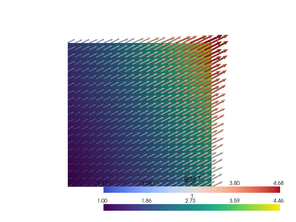
We can then plot the solutions, T and gh.
# plot T as a colormap
plotter_g = fenics_sz.utils.plot.plot_scalar(T, gather=True)
# plot g as glyphs
fenics_sz.utils.plot.plot_vector_glyphs(gh, plotter=plotter_g, gather=True, factor=0.03, cmap='coolwarm', scalar_bar_args={'title': '|grad T|'})
fenics_sz.utils.plot.plot_show(plotter_g)
fenics_sz.utils.plot.plot_save(plotter_g, output_folder / "2d_poisson_gradient.png")