Steady-State Subduction Zone Setup#
Implementation#
As a reminder our implementation is following a similar workflow to that seen in the background examples.
we will describe the subduction zone geometry and tesselate it into non-overlapping triangles to create a mesh
we will declare function spaces for the temperature, wedge velocity and pressure, and slab velocity and pressure
using these function spaces we will declare trial and test functions
we will define Dirichlet boundary conditions at the boundaries as described in the introduction
we will describe discrete weak forms for temperature and each of the coupled velocity-pressure systems that will be used to assemble the matrices (and vectors) to be solved
we will set up matrices and solvers for the discrete systems of equations
we will solve the matrix problems
We have now implemented all but the case-specific final step of solving the coupled velocity-pressure-temperature problem. In this notebook we do this for the case of steady-state, dislocation creep solutions, deriving a new SteadyDislSubductionProblem class from the SteadySubductionProblem class we implemented in notebooks/03_sz_problems/3.3a_sz_steady_problem.ipynb.
Preamble#
Let’s start by adding the path to the modules in the python folder to the system path (so we can find the our custom modules).
import sys, os, shutil
basedir = ''
if "__file__" in globals(): basedir = os.path.dirname(__file__)
sys.path.insert(0, os.path.join(basedir, os.path.pardir, os.path.pardir, 'python'))
Let’s also load the module generated by the previous notebooks to get access to the parameters, functions and classes defined there.
from fenics_sz.sz_problems.sz_params import default_params, allsz_params
from fenics_sz.sz_problems.sz_slab import create_slab
from fenics_sz.sz_problems.sz_geometry import create_sz_geometry
from fenics_sz.sz_problems.sz_problem import StokesSolverNest, TemperatureSolver
from fenics_sz.sz_problems.sz_steady_problem import SteadySubductionProblem
from fenics_sz.sz_problems.sz_steady_isoviscous import plot_slab_temperatures
Then let’s load all the required modules at the beginning.
import fenics_sz.geometry as geo
import fenics_sz.utils
from mpi4py import MPI
import dolfinx as df
import dolfinx.fem.petsc
from petsc4py import PETSc
import numpy as np
import scipy as sp
import ufl
import basix.ufl as bu
import matplotlib.pyplot as pl
import copy
import pyvista as pv
import pathlib
output_folder = pathlib.Path(os.path.join(basedir, "output"))
output_folder.mkdir(exist_ok=True, parents=True)
SteadyDislSubductionProblem class#
We build on the SteadySubductionProblem class implemented in notebooks/03_sz_problems/3.3a_sz_steady_problem.ipynb, deriving a SteadyDislSubductionProblem class that implements and solves the equations for a steady-state, dislocation creep case.
7. Solution#
Solving for the thermal state of the subduction zone is more complicated when using a dislocation creep viscosity than in the isoviscous rheology case due to the non-linearities introduced by having the viscosity depend on both temperature and velocity (through the strain rate). These mean that we must iterate between the velocity and temperature solutions until a (hopefully) converged solution is achieved. Due to the split nature of our submeshes we do this using a Picard or fixed-point iteration. These iterations are not guaranteed to converge but stand a much better chance with a good initial guess, so we start by solving the isoviscous problem again.
Given this initial guess, we test for convergence by calculating the residual of each subproblem and ensuring that their norm is small either in a relative (to the initial residual, rtol) or absolute (atol) sense. To prevent a runaway non-converging computation we place a maximum cap on the number of iterations (maxits). This iteration can take some time, particularly at high resolutions (low resscales).
To evaluate the residual norm we implement the function calculate_residual before using it in the solve function.
class SteadyDislSubductionProblem(SteadySubductionProblem):

    def calculate_residual(self, rw, rs, rT):
        """
        Given forms for the vpw, vps and T residuals,
        return the total residual of the problem.

        Arguments:
          * rw - residual form for the wedge velocity and pressure
          * rs - residual form for the slab velocity and pressure
          * rT - residual form for the temperature

        Returns:
          * r  - 2-norm of the combined residual
        """
        # because some of our forms are defined on different MPI comms
        # we need to calculate a squared 2-norm locally and use the global
        # comm to reduce it
        def calc_r_norm_sq(r, bcs, this_rank=True):
            r_norm_sq = 0.0
            if this_rank:
                r_vec = df.fem.petsc.assemble_vector_nest(r)
                # update the ghost values
                for r_vec_sub in r_vec.getNestSubVecs():
                    r_vec_sub.ghostUpdate(addv=PETSc.InsertMode.ADD, mode=PETSc.ScatterMode.REVERSE)
                # set bcs
                bcs_by_block = df.fem.bcs_by_block(df.fem.extract_function_spaces(r), bcs)
                df.fem.petsc.set_bc_nest(r_vec, bcs_by_block, alpha=0.0)
                r_arr = r_vec.getArray()
                r_norm_sq = np.inner(r_arr, r_arr)
            return r_norm_sq
        with df.common.Timer("Assemble Stokes"):
            r_norm_sq  = calc_r_norm_sq(rw, self.bcs_vw, self.wedge_rank)
            r_norm_sq += calc_r_norm_sq(rs, self.bcs_vs, self.slab_rank)
        self.comm.barrier()
        with df.common.Timer("Assemble Temperature"):
            r_norm_sq += calc_r_norm_sq(rT, self.bcs_T)
        r = self.comm.allreduce(r_norm_sq, op=MPI.SUM)**0.5
        return r

    def solve(self, rtol=5.e-6, atol=5.e-9, maxits=50,
              petsc_options_s=None, petsc_options_T=None):
        """
        Solve the Stokes problems assuming a dislocation creep rheology.

        Keyword Arguments:
          * rtol          - nonlinear iteration relative tolerance
          * atol          - nonlinear iteration absolute tolerance
          * maxits        - maximum number of nonlinear iterations
          * petsc_options_s - a dictionary of petsc options to pass to the Stokes solver
                              (defaults to an LU direct solver using the MUMPS library)
          * petsc_options_T - a dictionary of petsc options to pass to the temperature solver
                              (defaults to an LU direct solver using the MUMPS library)
        """
        # first solve the isoviscous problem
        self.solve_stokes_isoviscous(petsc_options=petsc_options_s)

        # retrieve the temperature forms (implemented in the parent class)
        ST, fT, rT = self.temperature_forms()
        solver_T = TemperatureSolver(ST, fT, self.bcs_T, self.T_i,
                                     petsc_options=petsc_options_T)
        # and solve the temperature problem, given the isoviscous Stokes solution
        self.T_i = solver_T.solve()
        self.update_T_functions()

        # retrieve the non-linear Stokes forms for the wedge
        Ssw, fsw, rsw, Msw = self.stokes_forms(self.wedge_vw_t, self.wedge_pw_t,
                                                self.wedge_vw_a, self.wedge_pw_a,
                                                self.wedge_vw_i, self.wedge_pw_i,
                                                eta=self.etadisl(self.wedge_vw_i, self.wedge_T_i))
        # set up a solver for the wedge velocity and pressure
        solver_s_w = StokesSolverNest(Ssw, fsw, self.bcs_vw,
                                      self.wedge_vw_i, self.wedge_pw_i,
                                      M=Msw, isoviscous=False,
                                      petsc_options=petsc_options_s)

        # retrieve the non-linear Stokes forms for the slab
        Sss, fss, rss, Mss = self.stokes_forms(self.slab_vs_t, self.slab_ps_t,
                                                self.slab_vs_a, self.slab_ps_a,
                                                self.slab_vs_i, self.slab_ps_i,
                                                eta=self.etadisl(self.slab_vs_i, self.slab_T_i))
        # set up a solver for the slab velocity and pressure
        solver_s_s = StokesSolverNest(Sss, fss, self.bcs_vs,
                                      self.slab_vs_i, self.slab_ps_i,
                                      M=Mss, isoviscous=False,
                                      petsc_options=petsc_options_s)

        # calculate the initial residual
        r = self.calculate_residual(rsw, rss, rT)
        r0 = r
        rrel = r/r0  # 1
        if self.comm.rank == 0:
            print("{:<11} {:<12} {:<17}".format('Iteration','Residual','Relative Residual'))
            print("-"*42)

        # iterate until the residual converges (hopefully)
        it = 0
        if self.comm.rank == 0: print("{:<11} {:<12.6g} {:<12.6g}".format(it, r, rrel,))
        while rrel > rtol and r > atol:
            if it > maxits: break
            # solve for v & p and interpolate the velocity
            if self.wedge_rank: self.wedge_vw_i, self.wedge_pw_i = solver_s_w.solve()
            if self.slab_rank:  self.slab_vs_i,  self.slab_ps_i  = solver_s_s.solve()
            self.update_v_functions()
            # wait for all ranks to catch up
            # (some may not have done anything above and
            # letting them carry on messes with profiling)
            self.comm.barrier()
            # solve for T and interpolate it
            self.T_i = solver_T.solve()
            self.update_T_functions()
            # calculate a new residual
            r = self.calculate_residual(rsw, rss, rT)
            rrel = r/r0
            it += 1
            if self.comm.rank == 0: print("{:<11} {:<12.6g} {:<12.6g}".format(it, r, rrel,))

        # check for convergence failures
        if it > maxits:
            raise Exception("Nonlinear iteration failed to converge after {} iterations (maxits = {}), r = {} (atol = {}), rrel = {} (rtol = {}).".format(it, \
                                                                                                                                                          maxits, \
                                                                                                                                                          r, \
                                                                                                                                                          rtol, \
                                                                                                                                                          rrel, \
                                                                                                                                                          rtol,))

        # only update the pressure at the end as it is not necessary earlier
        self.update_p_functions()
Demonstration - Benchmark case 2#
Our SteadyDislSubductionProblem class is now complete!
We demonstrate the new functionality using benchmark case 2. This uses a different io_depth (\(z_\text{io}\)) but otherwise has similar parameters to case 1 and we again use a low resolution demo (resscale = 5.0).
resscale = 5.0
xs = [0.0, 140.0, 240.0, 400.0]
ys = [0.0, -70.0, -120.0, -200.0]
lc_depth = 40
uc_depth = 15
coast_distance = 0
extra_width = 0
sztype = 'continental'
io_depth = 154.0
A      = 100.0      # age of subducting slab (Myr)
qs     = 0.065      # surface heat flux (W/m^2)
Vs     = 100.0      # slab speed (mm/yr)
slab = create_slab(xs, ys, resscale, lc_depth)
geom_case2 = create_sz_geometry(slab, resscale, sztype, io_depth, extra_width,
                                coast_distance, lc_depth, uc_depth)
sz_case2 = SteadyDislSubductionProblem(geom_case2, A=A, Vs=Vs, sztype=sztype, qs=qs)
This can then be used to solve case 2 and retrieve its diagnostics.
print("\nSolving steady state flow with dislocation creep rheology...")
sz_case2.solve()
Solving steady state flow with dislocation creep rheology...
Iteration   Residual     Relative Residual
------------------------------------------
0           14039.3      1
1           1161.26      0.0827153
2           256.735      0.0182869
3           103.968      0.0074055
4           48.9798      0.00348877
5           26.4549      0.00188435
6           16.1772      0.00115228
7           10.7653      0.0007668
8           7.60442      0.000541653
9           5.59295      0.000398379
10          4.21471      0.000300209
11          3.22359      0.000229612
12          2.4908       0.000177416
13          1.93954      0.000138151
14          1.51997      0.000108266
15          1.19783      8.53198e-05
16          0.948679     6.75732e-05
17          0.754764     5.37609e-05
18          0.602991     4.29503e-05
19          0.483598     3.44461e-05
20          0.389239     2.7725e-05
21          0.314337     2.23898e-05
22          0.254634     1.81372e-05
23          0.206858     1.47342e-05
24          0.168483     1.20008e-05
25          0.13755      9.79752e-06
26          0.112533     8.01558e-06
27          0.0922379    6.56999e-06
28          0.0757272    5.39395e-06
29          0.0622606    4.43474e-06
We can now resuse the routine defined previously to extract the diagnostic values.
diag_case2 = sz_case2.get_diagnostics()

print('')
print('{:<12} {:<12} {:<12} {:<12} {:<12} {:<12}'.format('resscale', 'T_ndof', 'T_{200,-100}', 'Tbar_s', 'Tbar_w', 'Vrmsw'))
print('{:<12.4g} {:<12d} {:<12.4f} {:<12.4f} {:<12.4f} {:<12.4f}'.format(resscale, *diag_case2.values()))
resscale     T_ndof       T_{200,-100} Tbar_s       Tbar_w       Vrmsw
5            5856         679.0166     568.5575     941.6615     41.9561
For comparison here are the values reported for case 2 using TerraFERMA in Wilson & van Keken, 2023:
|
\(T_{\text{ndof}} \) |
\(T_{(200,-100)}^*\) |
\(\overline{T}_s^*\) |
\( \overline{T}_w^* \) |
\(V_{\text{rms},w}^*\) |
|---|---|---|---|---|---|
2.0 |
21403 |
683.05 |
571.58 |
936.65 |
40.89 |
1.0 |
83935 |
682.87 |
572.23 |
936.11 |
40.78 |
0.5 |
332307 |
682.80 |
572.05 |
937.37 |
40.77 |
This time our solutions, though good, are not as accurate in the isoviscous case. We can investigate this by plotting the temperature and velocities.
plotter_dis = fenics_sz.utils.plot.plot_scalar(sz_case2.T_i, scale=sz_case2.T0, gather=True, cmap='coolwarm', scalar_bar_args={'title': 'Temperature (deg C)', 'bold':True})
fenics_sz.utils.plot.plot_vector_glyphs(sz_case2.vw_i, plotter=plotter_dis, factor=0.1, gather=True, color='k', scale=fenics_sz.utils.mps_to_mmpyr(sz_case2.v0))
fenics_sz.utils.plot.plot_vector_glyphs(sz_case2.vs_i, plotter=plotter_dis, factor=0.1, gather=True, color='k', scale=fenics_sz.utils.mps_to_mmpyr(sz_case2.v0))
sz_case2.geom.pyvistaplot(plotter=plotter_dis, color='green', width=2)
cdpt = sz_case2.geom.slab_spline.findpoint('Slab::FullCouplingDepth')
fenics_sz.utils.plot.plot_points([[cdpt.x, cdpt.y, 0.0]], plotter=plotter_dis, render_points_as_spheres=True, point_size=10.0, color='green')
fenics_sz.utils.plot.plot_show(plotter_dis)
fenics_sz.utils.plot.plot_save(plotter_dis, output_folder / "sz_problem_case2_solution.png")
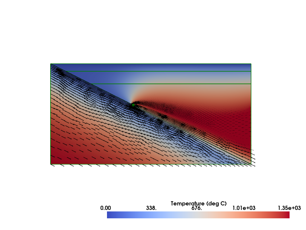
Where we can see that the wedge velocity is much more “pinched” near the coupling depth with the dislocation creep viscosity. This likely explains our poor performance in the benchmark at the low resolution we selected.
The output can also be saved to disk and opened with other visualization software (e.g. Paraview).
filename = output_folder / "sz_problem_case2_solution.bp"
with df.io.VTXWriter(sz_case2.mesh.comm, filename, [sz_case2.T_i, sz_case2.vs_i, sz_case2.vw_i]) as vtx:
    vtx.write(0.0)
# zip the .bp folder so that it can be downloaded from jupyter lab
shutil.make_archive(str(filename), 'zip', root_dir=str(filename.parent), base_dir=str(filename.name))
'/__w/fenics-sz/fenics-sz/notebooks/03_sz_problems/output/sz_problem_case2_solution.bp.zip'
We can also now project and visualize the dislocation-creep viscosity (note that we are using a log scale) to see the cause of the flow restriction in this case.
eta_i = sz_case2.project_dislocationcreep_viscosity()
plotter_eta = fenics_sz.utils.plot.plot_scalar(eta_i, scale=sz_case2.eta0, log_scale=True, show_edges=True, scalar_bar_args={'title': 'Viscosity (Pa s) [log scale]', 'bold':True})
sz_case2.geom.pyvistaplot(plotter=plotter_eta, color='green', width=2)
cdpt = sz_case2.geom.slab_spline.findpoint('Slab::FullCouplingDepth')
fenics_sz.utils.plot.plot_points([[cdpt.x, cdpt.y, 0.0]], plotter=plotter_eta, render_points_as_spheres=True, point_size=10.0, color='green')
fenics_sz.utils.plot.plot_show(plotter_eta)
fenics_sz.utils.plot.plot_save(plotter_eta, output_folder / "sz_problem_case2_eta.png")
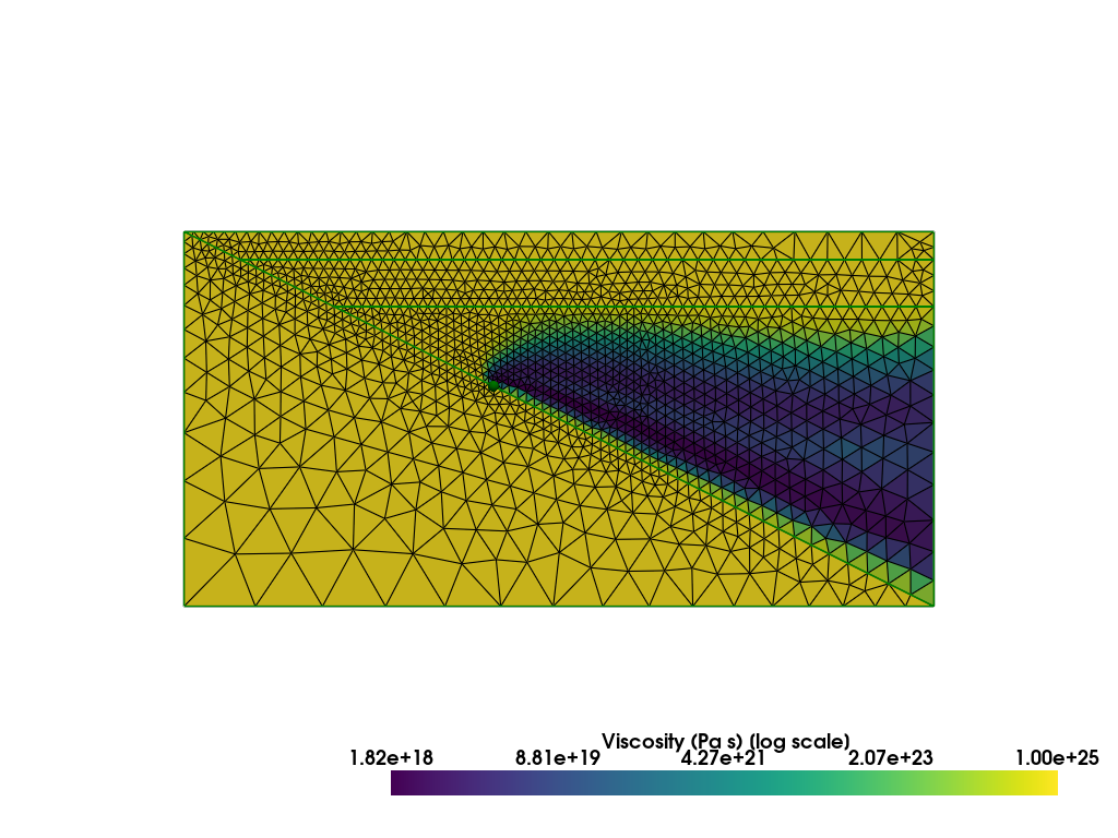
Clearly the velocity is constrained by the much higher viscosities in the low temperature or low strain rate regions of the domain.
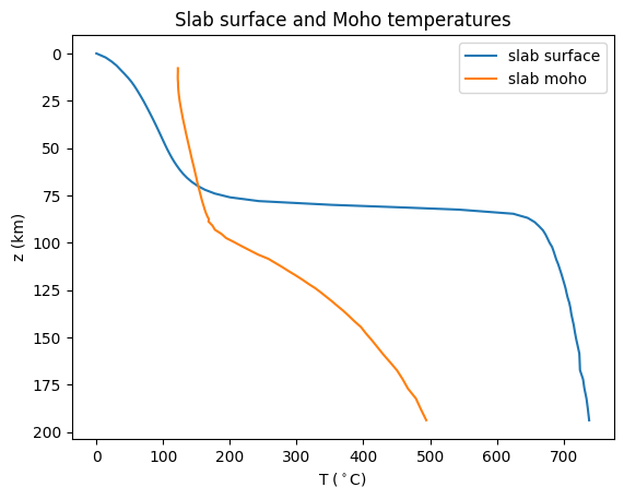
We can also reuse our slab temperature function to see their behavior in case 2.
fig = plot_slab_temperatures(sz_case2)
fig.savefig(output_folder / "sz_problem_case2_slabTs.png")
Themes and variations#
We now have a working implementation of a steady state subduction zone model. Some possible things to try next:
Try using
plot_slab_temperaturesas a template to extract different temperatures around the domain. Perhaps a vertical profile under a putative arc location.Note that at the default resolution in this notebook case 2 did not do as well as case 1 at matching the benchmark. Try increasing the resolution to see if it improves the solution (if running on binder then it may not be possible to decrease
resscaleexcessively).Try varying aspects of the geometry. What happens at different slab dips or when
extra_width > 0?Try varying some of the optional parameters, such as the coupling depth,
coupling_depth.
Even though this notebook set up the benchmark problem it should be valid for any of the global suite discussed in van Keken & Wilson, 2023, which is itself built on the suite in Syracuse et al., 2010. Try running a steady-state version of one of those cases using the parameters in allsz_params (from sz_params, which loaded the data in data/all_sz.json).