Batchelor Cornerflow Example#
Description#
As a reminder we are seeking the approximate velocity and pressure solution of the Stokes equation
in a unit square domain, \(\Omega = [0,1]\times[0,1]\).
We apply strong Dirichlet boundary conditions for velocity on all four boundaries
and a constraint on the pressure to remove its null space, e.g. by applying a reference point
Implementation#
The solution to this example was presented in Batchelor (1967) and has been used frequently as a benchmark problem. One such implementation was presented by Wilson & van Keken, 2023 using TerraFERMA, a GUI-based model building framework that uses FEniCS v2019.1.0. Here we reproduce these results using the latest version of FEniCS, FEniCSx.
Preamble#
We start by loading all the modules we will require.
from mpi4py import MPI
import dolfinx as df
import dolfinx.fem.petsc
from petsc4py import PETSc
import numpy as np
import ufl
import matplotlib.pyplot as pl
import basix
import sys, os
basedir = ''
if "__file__" in globals(): basedir = os.path.dirname(__file__)
sys.path.insert(0, os.path.join(basedir, os.path.pardir, os.path.pardir, 'python'))
import fenics_sz.utils.plot
import pathlib
output_folder = pathlib.Path(os.path.join(basedir, "output"))
output_folder.mkdir(exist_ok=True, parents=True)
Solution#
We start by defining the analytical solution
where \(\psi = \psi(r,\theta)\) is a function of the radius, \(r\), and angle from the \(x\)-axis, \(\theta\)
We describe this solution using UFL in the python function v_exact_batchelor.
def v_exact_batchelor(mesh, U=1):
    """
    A python function that returns the exact Batchelor velocity solution
    using UFL on the given mesh.
    Parameters:
    * mesh - the mesh on which we wish to define the coordinates for the solution
    * U    - convergence speed of lower boundary (defaults to 1)
    """
    # Define the coordinate systems
    x = ufl.SpatialCoordinate(mesh)
    theta = ufl.atan2(x[1],x[0])

    # Define the derivative to the streamfunction psi
    d_psi_d_r = -U*(-0.25*ufl.pi**2*ufl.sin(theta) \
                    +0.5*ufl.pi*theta*ufl.sin(theta) \
                    +theta*ufl.cos(theta)) \
                    /(0.25*ufl.pi**2-1)
    d_psi_d_theta_over_r = -U*(-0.25*ufl.pi**2*ufl.cos(theta) \
                               +0.5*ufl.pi*ufl.sin(theta) \
                               +0.5*ufl.pi*theta*ufl.cos(theta) \
                               +ufl.cos(theta) \
                               -theta*ufl.sin(theta)) \
                               /(0.25*ufl.pi**2-1)

    # Rotate the solution into Cartesian and return
    return ufl.as_vector([ufl.cos(theta)*d_psi_d_theta_over_r + ufl.sin(theta)*d_psi_d_r, \
                          ufl.sin(theta)*d_psi_d_theta_over_r - ufl.cos(theta)*d_psi_d_r])
We then build a workflow that contains a complete description of the discrete Stokes equation problem. This follows much the same flow as described in previous examples but because this case is more complicated we split up each step into individual functions that we combine later into a single function call
in
unit_square_meshwe describe the unit square domain \(\Omega = [0,1]\times[0,1]\) and discretize it into \(2 \times\)ne\(\times\)netriangular elements or cells to make amesh
def unit_square_mesh(ne):
    """
    A python function to set up a mesh of a unit square domain.
    Parameters:
    * ne   - number of elements in each dimension
    Returns:
    * mesh - the mesh
    """
    # Describe the domain (a unit square)
    # and also the tessellation of that domain into ne
    # equally spaced squared in each dimension, which are
    # subduvided into two triangular elements each
    with df.common.Timer("Mesh"):
        mesh = df.mesh.create_unit_square(MPI.COMM_WORLD, ne, ne,
                                          ghost_mode=df.mesh.GhostMode.none)
    return mesh
in
functionspaceswe declare finite elements for velocity and pressure using Lagrange polynomials of degreep+1andprespectively and use these to declare the function spaces,V_vandV_p, for velocity and pressure respectively
def functionspaces(mesh, p=1):
    """
    A python function to set up velocity and pressure function spaces.
    Parameters:
    * mesh - the mesh to set up the functions on
    * p    - polynomial order of the pressure solution (optional, defaults to 1)
    Returns:
    * V_v  - velocity function space of polynomial order p+1
    * V_p  - pressure function space of polynomial order p
    """
    with df.common.Timer("Function spaces"):
        # Define velocity and pressure elements
        v_e = basix.ufl.element("Lagrange", mesh.basix_cell(), p+1, shape=(mesh.geometry.dim,))
        p_e = basix.ufl.element("Lagrange", mesh.basix_cell(), p)

        # Define the velocity and pressure function spaces
        V_v = df.fem.functionspace(mesh, v_e)
        V_p = df.fem.functionspace(mesh, p_e)

    return V_v, V_p
set up boundary conditions
in
velocity_bcswe define a list of Dirichlet boundary conditions on velocityin
pressure_bcswe define a constraint on the pressure in the lower left corner of the domain
def velocity_bcs(V_v, U=1):
    """
    A python function to set up the velocity boundary conditions.
    Parameters:
    * V_v - velocity function space
    * U   - convergence speed of lower boundary (optional, defaults to 1)
    Returns:
    * bcs - a list of boundary conditions
    """
    with df.common.Timer("Dirichlet BCs"):
        # Declare a list of boundary conditions
        bcs = []

        # Grab the mesh
        mesh = V_v.mesh

        # Define the location of the left boundary and find the velocity DOFs
        def boundary_left(x):
            return np.isclose(x[0], 0)
        dofs_v_left = df.fem.locate_dofs_geometrical(V_v, boundary_left)
        # Specify the velocity value and define a Dirichlet boundary condition
        zero_v = df.fem.Constant(mesh, df.default_scalar_type((0.0, 0.0)))
        bcs.append(df.fem.dirichletbc(zero_v, dofs_v_left, V_v))

        # Define the location of the bottom boundary and find the velocity DOFs
        # for x velocity (0) and y velocity (1) separately
        def boundary_base(x):
            return np.isclose(x[1], 0)
        dofs_v_base = df.fem.locate_dofs_geometrical(V_v, boundary_base)
        # Specify the value of the x component of velocity and define a Dirichlet boundary condition
        U_v = df.fem.Constant(mesh, df.default_scalar_type((U, 0.0)))
        bcs.append(df.fem.dirichletbc(U_v, dofs_v_base, V_v))

        # Define the location of the right and top boundaries and find the velocity DOFs
        def boundary_rightandtop(x):
            return np.logical_or(np.isclose(x[0], 1), np.isclose(x[1], 1))
        dofs_v_rightandtop = df.fem.locate_dofs_geometrical(V_v, boundary_rightandtop)
        # Specify the exact velocity value and define a Dirichlet boundary condition
        exact_v = df.fem.Function(V_v)
        # Interpolate from a UFL expression, evaluated at the velocity interpolation points
        exact_v.interpolate(df.fem.Expression(v_exact_batchelor(mesh, U=U), V_v.element.interpolation_points()))
        bcs.append(df.fem.dirichletbc(exact_v, dofs_v_rightandtop))

    return bcs

def pressure_bcs(V_p):
    """
    A python function to set up the pressure boundary conditions.
    Parameters:
    * V_p - pressure function space
    Returns:
    * bcs - a list of boundary conditions
    """
    with df.common.Timer("Dirichlet BCs"):
        # Declare a list of boundary conditions
        bcs = []

        # Grab the mesh
        mesh = V_p.mesh

        # Define the location of the lower left corner of the domain and find the pressure DOF there
        def corner_lowerleft(x):
            return np.logical_and(np.isclose(x[0], 0), np.isclose(x[1], 0))
        dofs_p_lowerleft = df.fem.locate_dofs_geometrical(V_p, corner_lowerleft)
        # Specify the arbitrary pressure value and define a Dirichlet boundary condition
        zero_p = df.fem.Constant(mesh, df.default_scalar_type(0.0))
        bcs.append(df.fem.dirichletbc(zero_p, dofs_p_lowerleft, V_p))

    return bcs
declare discrete weak forms
stokes_weakformsuses the velocity and pressure function spaces to declare trial,v_aandp_a, and test,v_tandp_t, functions for the velocity and pressure respectively and uses them to describe the discrete weak forms,Sandf, that will be used to assemble the matrix \(\mathbf{A}\) and vector \(\mathbf{b}\)we also implement a dummy weak form for the pressure block in
dummy_pressure_weakformthat allows us to apply a pressure boundary condition
def stokes_weakforms(V_v, V_p):
    """
    A python function to return the weak forms of the Stokes problem.
    Parameters:
    * V_v - velocity function space
    * V_p - pressure function space
    Returns:
    * S   - a bilinear form
    * f   - a linear form
    """
    with df.common.Timer("Forms"):
        # Grab the mesh
        mesh = V_p.mesh

        # Define the trial functions for velocity and pressure
        v_a, p_a = ufl.TrialFunction(V_v), ufl.TrialFunction(V_p)
        # Define the test functions for velocity and pressure
        v_t, p_t = ufl.TestFunction(V_v),  ufl.TestFunction(V_p)

        # Define the integrals to be assembled into the stiffness matrix
        K = ufl.inner(ufl.sym(ufl.grad(v_t)), ufl.sym(ufl.grad(v_a))) * ufl.dx
        G = -ufl.div(v_t)*p_a*ufl.dx
        D = -p_t*ufl.div(v_a)*ufl.dx
        S = df.fem.form([[K, G], [D, None]])

        # Define the integral to the assembled into the forcing vector
        # which in this case is just zero
        zero_p = df.fem.Constant(mesh, df.default_scalar_type(0.0))
        zero_v = df.fem.Constant(mesh, df.default_scalar_type((0.0, 0.0)))
        f = df.fem.form([ufl.inner(v_t, zero_v)*ufl.dx, zero_p*p_t*ufl.dx])

    return S, f

def dummy_pressure_weakform(V_p):
    """
    A python function to return a dummy (zero) weak form for the pressure block of
    the Stokes problem.
    Parameters:
    * V_p - pressure function space
    Returns:
    * M   - a bilinear form
    """
    with df.common.Timer("Forms"):
        # Grab the mesh
        mesh = V_p.mesh

        # Define the trial function for the pressure
        p_a = ufl.TrialFunction(V_p)
        # Define the test function for the pressure
        p_t = ufl.TestFunction(V_p)

        # Define the dummy integrals to be assembled into a zero pressure mass matrix
        zero_p = df.fem.Constant(mesh, df.default_scalar_type(0.0))
        M = df.fem.form(p_t*p_a*zero_p*ufl.dx)

    return M
in
assemblewe assemble the matrix problem
def assemble(S, f, bcs):
    """
    A python function to assemble the forms into a matrix and a vector.
    Parameters:
    * S   - Stokes form
    * f   - RHS form
    * bcs - list of boundary conditions
    Returns:
    * Sm  - a matrix
    * fm  - a vector
    """
    with df.common.Timer("Assemble"):
        Sm = df.fem.petsc.assemble_matrix_block(S, bcs=bcs)
        Sm.assemble()
        fm = df.fem.petsc.assemble_vector_block(f, S, bcs=bcs)
    return Sm, fm
in
solvewe solve the matrix problem using a PETSc linear algebra back-end, returning the solution functions for velocity,v_i, and pressure,p_i
def solve(Sm, fm, V_v, V_p):
    """
    A python function to solve a matrix vector system.
    Parameters:
    * Sm  - matrix
    * fm  - vector
    * V_v - velocity function space
    * V_p - pressure function space
    Returns:
    * v_i - velocity solution function
    * p_i - pressure solution function
    """

    with df.common.Timer("Solve"):
        solver = PETSc.KSP().create(MPI.COMM_WORLD)
        solver.setOperators(Sm)
        solver.setFromOptions()

        # Create a solution vector and solve the system
        x = Sm.createVecRight()
        solver.solve(fm, x)

        # Set up the solution functions
        v_i = df.fem.Function(V_v)
        p_i = df.fem.Function(V_p)
        # Extract the velocity and pressure solutions for the coupled problem
        offset = V_v.dofmap.index_map.size_local*V_v.dofmap.index_map_bs
        v_i.x.array[:offset] = x.array_r[:offset]
        p_i.x.array[:(len(x.array_r) - offset)] = x.array_r[offset:]
        # Update the ghost values
        v_i.x.scatter_forward()
        p_i.x.scatter_forward()

    with df.common.Timer("Cleanup"):
        solver.destroy()
        x.destroy()

    return v_i, p_i
Finally, we set up a python function, solve_batchelor, that brings all these steps together into a complete problem.
def solve_batchelor(ne, p=1, U=1, petsc_options=None):
    """
    A python function to solve a two-dimensional corner flow
    problem on a unit square domain.
    Parameters:
    * ne - number of elements in each dimension
    * p  - polynomial order of the pressure solution (optional, defaults to 1)
    * U  - convergence speed of lower boundary (optional, defaults to 1)
    * petsc_options - a dictionary of petsc options to pass to the solver
                      (optional, defaults to an LU direct solver using the MUMPS library)
    Returns:
    * v_i - velocity solution function
    * p_i - pressure solution function
    """

    # 0. Set some default PETSc options
    if petsc_options is None:
        petsc_options = {"ksp_type": "preonly", \
                         "pc_type": "lu",
                         "pc_factor_mat_solver_type": "mumps"}
    # and load them into the PETSc options system
    opts = PETSc.Options()
    for k, v in petsc_options.items(): opts[k] = v

    # 1. Set up a mesh
    mesh = unit_square_mesh(ne)
    # 2. Declare the appropriate function spaces
    V_v, V_p = functionspaces(mesh, p)
    # 3. Collect all the boundary conditions into a list
    bcs  = velocity_bcs(V_v, U=U)
    bcs += pressure_bcs(V_p)
    # 4. Declare the weak forms
    S, f = stokes_weakforms(V_v, V_p)
    #    Include a dummy zero pressure mass matrix to allow us to set a pressure constraint
    S[1][1] = dummy_pressure_weakform(V_p)
    # 5. Assemble the matrix equation
    Sm, fm = assemble(S, f, bcs)
    # 6. Solve the matrix equation
    v_i, p_i = solve(Sm, fm, V_v, V_p)

    with df.common.Timer("Cleanup"):
        Sm.destroy()
        fm.destroy()

    return v_i, p_i
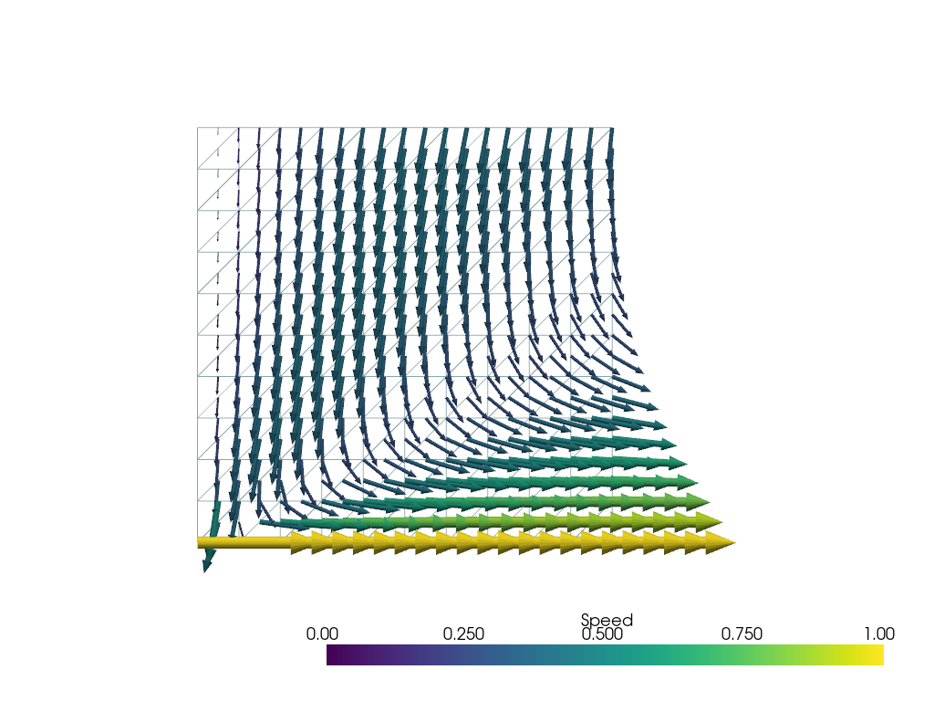
We can now numerically solve the equations using, e.g., 10 elements in each dimension and piecewise linear polynomials for pressure (and piecewise quadratic polynomials for velocity).
ne = 10
p = 1
U = 1
v, p = solve_batchelor(ne, p=p, U=U)
v.name = "Velocity"
And use some utility functions (see python/fenics_sz/utils/plot.py) to plot it.
plotter = fenics_sz.utils.plot.plot_mesh(v.function_space.mesh, gather=True, show_edges=True, style="wireframe")
fenics_sz.utils.plot.plot_vector_glyphs(v, plotter=plotter, gather=True, factor=0.3, scalar_bar_args={'title': 'Speed'})
fenics_sz.utils.plot.plot_show(plotter)
fenics_sz.utils.plot.plot_save(plotter, output_folder / 'batchelor_solution.png')
Testing#
Error analysis#
We can quantify the error in cases where the analytical solution is known by taking the L2 norm of the difference between the numerical and exact solutions.
def evaluate_error(v_i, U=1):
    """
    A python function to evaluate the l2 norm of the error in
    the two dimensional Batchelor corner flow problem.
    Parameters:
    * v_i - numerical solution for velocity
    * U   - convergence speed of lower boundary (optional, defaults to 1)
    Returns:
    * l2err - l2 error of solution
    """
    # Define the exact solution (in UFL)
    ve = v_exact_batchelor(v_i.function_space.mesh, U=U)

    # Define the error as the squared difference between the exact solution and the given approximate solution
    l2err = df.fem.assemble_scalar(df.fem.form(ufl.inner(v_i - ve, v_i - ve)*ufl.dx))
    l2err = v_i.function_space.mesh.comm.allreduce(l2err, op=MPI.SUM)**0.5

    # Return the l2 norm of the error
    return l2err
Convergence test#
Repeating the numerical experiments with increasing ne allows us to test the convergence of our approximate finite element solution to the known analytical solution. A key feature of any discretization technique is that with an increasing number of degrees of freedom (DOFs) these solutions should converge, i.e. the error in our approximation should decrease.
We implement a function, convergence_errors to loop over different pressure polynomial orders, p, and numbers of elements, ne evaluating the error for each.
def convergence_errors(ps, nelements, U=1, petsc_options=None):
    """
    A python function to run a convergence test of a two-dimensional corner flow
    problem on a unit square domain.
    Parameters:
    * ps        - a list of pressure polynomial orders to test
    * nelements - a list of the number of elements to test
    * U         - convergence speed of lower boundary (optional, defaults to 1)
    * petsc_options - a dictionary of petsc options to pass to the solver
                      (optional, defaults to an LU direct solver using the MUMPS library)
    Returns:
    * errors_l2 - a list of l2 errors
    """
    errors_l2 = []
    # Loop over the polynomial orders
    for p in ps:
        # Accumulate the errors
        errors_l2_p = []
        # Loop over the resolutions
        for ne in nelements:
            # Solve the 2D Batchelor corner flow problem
            v_i, p_i = solve_batchelor(ne, p=p, U=U,
                                       petsc_options=petsc_options)
            # Evaluate the error in the approximate solution
            l2error = evaluate_error(v_i, U=U)
            # Print to screen and save if on rank 0
            if MPI.COMM_WORLD.rank == 0:
                print('p={}, ne={}, l2error={}'.format(p, ne, l2error))
            errors_l2_p.append(l2error)
        if MPI.COMM_WORLD.rank == 0:
            print('*************************************************')
        errors_l2.append(errors_l2_p)

    return errors_l2
We can use this function to get the errors at a range of polynomial orders and numbers of elements.
# List of polynomial orders to try
ps = [1, 2]
# List of resolutions to try
nelements = [10, 20, 40, 80, 160]

errors_l2 = convergence_errors(ps, nelements)
p=1, ne=10, l2error=0.021921089471662037
p=1, ne=20, l2error=0.010960435556187075
p=1, ne=40, l2error=0.005480211135211741
p=1, ne=80, l2error=0.0027401051388757816
p=1, ne=160, l2error=0.0013700525406580791
*************************************************
p=2, ne=10, l2error=0.012877716729228609
p=2, ne=20, l2error=0.0064388586951979665
p=2, ne=40, l2error=0.003219429351274253
p=2, ne=80, l2error=0.0016097146756471187
p=2, ne=160, l2error=0.0008048573378448104
*************************************************
Here we can see that the error is decreasing both with increasing ne and increasing p but this is clearer if we plot the errors and evaluate their order of convergence. To do this we write a python function test_plot_convergence.
def test_plot_convergence(ps, nelements, errors_l2, output_basename=None):
    """
    A python function to test and plot convergence of the given errors.
    Parameters:
    * ps              - a list of pressure polynomial orders to test
    * nelements       - a list of the number of elements to test
    * errors_l2       - errors_l2 from convergence_errors
    * output_basename - basename for output (optional, defaults to no output)
    Returns:
    * test_passes     - a boolean indicating if the convergence test has passed
    """

    # Open a figure for plotting
    if MPI.COMM_WORLD.rank == 0:
        fig = pl.figure()
        ax = fig.gca()

    # Keep track of whether we get the expected order of convergence
    test_passes = True

    # Loop over the polynomial orders
    for i, p in enumerate(ps):
        # Work out the order of convergence at this p
        hs = 1./np.array(nelements)/p
        # Fit a line to the convergence data
        fit = np.polyfit(np.log(hs), np.log(errors_l2[i]),1)
        # Test if the order of convergence is as expected (first order)
        test_passes = test_passes and abs(fit[0]-1) < 0.1

        # Write the errors to disk
        if MPI.COMM_WORLD.rank == 0:
            if output_basename is not None:
                with open(str(output_basename) + '_p{}.csv'.format(p), 'w') as f:
                    np.savetxt(f, np.c_[nelements, hs, errors_l2[i]], delimiter=',',
                             header='nelements, hs, l2errs')

            print("order of accuracy p={}, order={}".format(p,fit[0]))

            # log-log plot of the L2 error
            ax.loglog(hs,errors_l2[i],'o-',label='p={}, order={:.2f}'.format(p,fit[0]))

    if MPI.COMM_WORLD.rank == 0:
        # Tidy up the plot
        ax.set_xlabel(r'$h$')
        ax.set_ylabel(r'$||e||_2$')
        ax.grid()
        ax.set_title('Convergence')
        ax.legend()

        # Write convergence to disk
        if output_basename is not None:
            fig.savefig(str(output_basename) + '.pdf')

            print("***********  convergence figure in "+str(output_basename)+".pdf")

    return test_passes
test_passes = test_plot_convergence(ps, nelements, errors_l2,
                                    output_basename=output_folder / 'batchelor_convergence')

assert(test_passes)
order of accuracy p=1, order=1.0000034726074625
order of accuracy p=2, order=0.9999999846814445
*********** convergence figure in output/batchelor_convergence.pdf
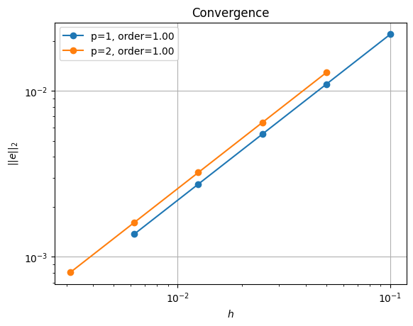
Solving the equations on a series of successively finer meshes and comparing the resulting solution to the analytical result using the error metric
shows linear rather than quadratic convergence, regardless of the polynomial order we select for our numerical solution.
This first-order convergence rate is lower than would be expected for piecewise quadratic or piecewise cubic velocity functions (recall that the velocity is one degree higher than the specified pressure polynomial degree). This drop in convergence rate is caused by the boundary conditions at the origin being discontinuous, which cannot be represented in the selected function space and results in a pressure singularity at that point. This is an example where convergence analysis demonstrates suboptimal results due to our inability to represent the solution in the selected finite element function space.
Aside from the convergence rate we are also interested in the performance of our implementation. We will test this in the next notebook by timing different sections of our calculation both in serial and parallel.