Batchelor Cornerflow Example#
Description#
As a reminder we are seeking the approximate velocity and pressure solution of the Stokes equation
in a unit square domain, \(\Omega = [0,1]\times[0,1]\).
We apply strong Dirichlet boundary conditions for velocity on all four boundaries
and a constraint on the pressure to remove its null space, e.g. by applying a reference point
Parallel Scaling#
In the previous notebook we tested that the solution of the Batchelor cornerflow problem using our new implementation of the Stokes equation, using a PETSc MATNEST matrix, converged at the same suboptimal rate as our original implementation. We also wish to test for parallel scaling of the new implementation, assessing if the simulation wall time decreases as the number of processors used to solve it is increases.
Here we perform strong scaling tests on our function solve_batchelor_nest from notebooks/02_background/2.4d_batchelor_nest.ipynb.
Preamble#
We start by loading all the modules we will require.
import sys, os
basedir = ''
if "__file__" in globals(): basedir = os.path.dirname(__file__)
path = os.path.join(basedir, os.path.pardir, os.path.pardir, 'python')
sys.path.insert(0, path)
import fenics_sz.utils.ipp
from fenics_sz.background.batchelor import test_plot_convergence
import matplotlib.pyplot as pl
import matplotlib.ticker as ticker
import numpy as np
import pathlib
output_folder = pathlib.Path(os.path.join(basedir, "output"))
output_folder.mkdir(exist_ok=True, parents=True)
Implementation#
We perform the strong parallel scaling test using a utility function (profile_parallel from python/utils/ipp.py) that loops over a list of the number of processors calling our function for a given number of elements, ne, and polynomial order p. It runs our function solve_batchelor a specified number of times and evaluates and returns the time taken for each of a number of requested steps.
# the list of the number of processors we will use
nprocs_scale = [1, 2, 4]

# the number of elements in each direction (total elements = 2*ne*ne)
ne = 128

# the polynomial degree of our pressure field
p = 1

# perform the calculation a set number of times
number = 10

# We are interested in the time to create the mesh,
# declare the functions, assemble the problem and solve it.
# From our implementation in `solve_poisson_2d` it is also
# possible to request the time to declare the Dirichlet and
# Neumann boundary conditions and the forms.
steps = [
          'Mesh', 'Function spaces',
          'Assemble', 'Solve',
         ]

# declare a dictionary to store the times each step takes
maxtimes = {}
Direct (block)#
To start with we test the scaling with the original implementation and the default solver options, which are a direct LU decomposition using the MUMPS library implementation.
petsc_options = {'ksp_type' : 'preonly', 'pc_type' : 'lu', 'pc_factor_mat_solver_type' : 'mumps', 'mat_mumps_icntl_4': 2}

def extra_parallel_diagnostics(out):
    v = out[0]
    p = out[1]
    diag = dict()
    bs = v.function_space.dofmap.index_map_bs
    diag['v_ndofs']   = v.function_space.dofmap.index_map.size_local*bs
    diag['v_nghosts'] = v.function_space.dofmap.index_map.num_ghosts*bs
    diag['p_ndofs']   = p.function_space.dofmap.index_map.size_local
    diag['p_nghosts'] = p.function_space.dofmap.index_map.num_ghosts
    return diag

maxtimes_db, maxmumpstimes_db, extradiagout_db  = fenics_sz.utils.ipp.profile_parallel(nprocs_scale, steps, path, 'fenics_sz.background.batchelor', 'solve_batchelor',
                                                        ne, p, number=number, include_mumps_times=True,
                                                        extra_diagnostics_func=extra_parallel_diagnostics,
                                                        petsc_options=petsc_options,
                                                        output_filename=output_folder / 'batchelor_scaling_direct_block.png')

maxtimes['Direct (block)'] = maxtimes_db
=========================
                     1           2           4
Mesh                 0.026       0.035       0.053
Function spaces      0.02        0.014       0.017
Assemble             0.25        0.148       0.129
Solve                1.419       1.232       1.424
=========================
MUMPS analysis       0.70875     0.72125     0.89612
MUMPS factorization  0.65776     0.46046     0.4824
MUMPS solve          0.04544     0.03124     0.02781
=========================
v_ndofs_max          132098      66160       33208
v_ndofs_min          132098      65938       32728
v_ndofs_sum          132098      132098      132098
v_ndofs_avg          132098      66049       33024.5
v_nghosts_max        0           282         376
v_nghosts_min        0           232         244
v_nghosts_sum        0           514         1158
v_nghosts_avg        0           257         289.5
p_ndofs_max          16641       8329        4190
p_ndofs_min          16641       8312        4128
p_ndofs_sum          16641       16641       16641
p_ndofs_avg          16641       8320.5      4160.25
p_nghosts_max        0           71          94
p_nghosts_min        0           58          63
p_nghosts_sum        0           129         291
p_nghosts_avg        0           64.5        72.75
=========================
*********** profiling figure in output/batchelor_scaling_direct_block.png
The behavior of the scaling test will strongly depend on the computational resources available on the machine where this notebook is run. In particular when the website is generated it has to run as quickly as possible on github, hence we limit our requested numbers of processors, size of the problem (ne and p) and number of calculations to average over (number) in the default setup of this notebook.
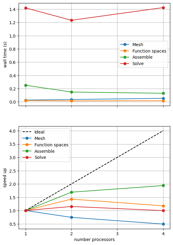
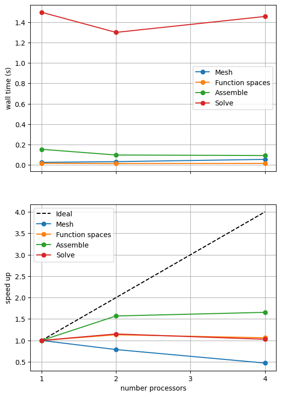
For comparison we provide the output of this notebook using ne = 256, p = 1 and number = 10 in Figure 2.4.2 generated on a dedicated machine with a local conda installation of the software.
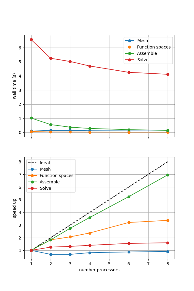
Figure 2.4.2 Scaling results for a direct solver with ne = 256, p = 1 averaged over number = 10 calculations using a local conda installation of the software on a dedicated machine.
We can see in Figure 2.4.2 that assembly and function space declarations scale well, with assembly being almost ideal. However meshing and the solve barely scale at all. As previously discussed, the meshing takes place on a single process before being communicated to the other processors, hence we do not expect this step to scale. Additionally the cost (wall time taken) of meshing is so small that it is not a significant factor in these simulations. The solution step is our most significant cost and would ideally scale.
We can also see how different parts of the poorly scaling solution step scale individually by looking at the analysis, factorization and solve steps of the MUMPS solver.
fig, (ax, ax_r) = pl.subplots(nrows=2, figsize=[6.4,9.6], sharex=True)
for k in maxmumpstimes_db[0].keys():
    ax.plot(nprocs_scale, [maxtimes[k] for maxtimes in maxmumpstimes_db], 'o-', label=k)
ax.xaxis.set_major_locator(ticker.MaxNLocator(integer=True))
ax.set_ylabel('wall time (s)')
ax.grid()
ax.legend()

ax_r.plot(nprocs_scale, [nproc/nprocs_scale[0] for nproc in nprocs_scale], 'k--', label='Ideal')
for k in maxmumpstimes_db[0].keys():
    ax_r.plot(nprocs_scale, maxmumpstimes_db[0][k]/np.asarray([maxtimes[k] for maxtimes in maxmumpstimes_db]), 'o-', label=k)
ax_r.xaxis.set_major_locator(ticker.MaxNLocator(integer=True))
ax_r.set_xlabel('number processors')
ax_r.set_ylabel('speed up')
ax_r.grid()
ax_r.legend()

fig.savefig(output_folder / 'batchelor_scaling_direct_block_mumps.png')
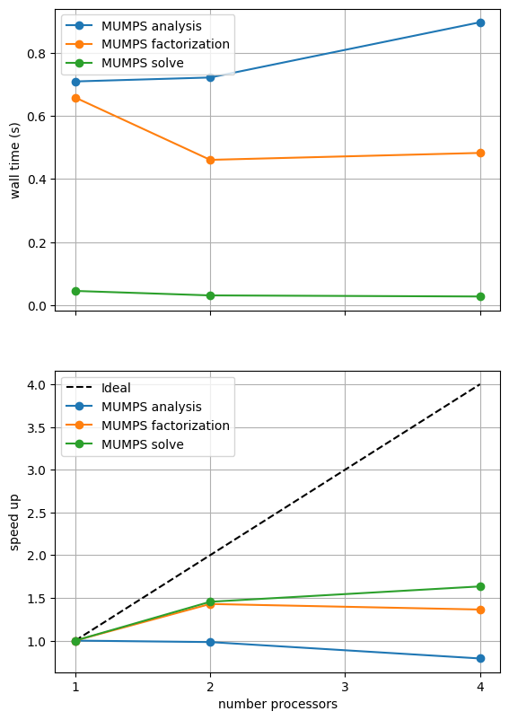
What the above result shows will depend on the machine it is run on (and is unlikely to look perform well during website generation) so we present a previously computed result using ne = 256, p = 1 and number = 10 in Figure 2.4.3 generated on a dedicated machine with a local conda installation of the software.
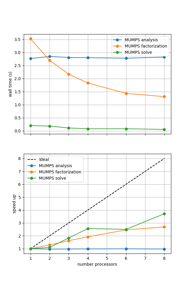
Figure 2.4.3 MUMPS scaling results for a direct solver with ne = 256, p = 1 averaged over number = 10 calculations using a local conda installation of the software on a dedicated machine.
As before in the Poisson example we see that the analysis step does not scale at all (as, by default, it is performed on a single process) while the factorization and solution steps do scale (although quite poorly).
One factor contributing to poor scaling at large numbers of processes is the increased communication cost. We can look at one measure of this by plotting the numbers of degrees of freedom on each process and the total number of ghost degrees of freedom.
fig, (ax, ax_r) = pl.subplots(nrows=2, figsize=[6.4,9.6], sharex=True)

v_ndofs_avg = np.asarray([extradiag['v_ndofs_avg'] for extradiag in extradiagout_db])
v_ndofs_min = np.asarray([extradiag['v_ndofs_min'] for extradiag in extradiagout_db])
v_ndofs_max = np.asarray([extradiag['v_ndofs_max'] for extradiag in extradiagout_db])
v_ndofs_errs = [np.abs(v_ndofs_min-v_ndofs_avg), np.abs(v_ndofs_max-v_ndofs_avg)]

p_ndofs_avg = np.asarray([extradiag['p_ndofs_avg'] for extradiag in extradiagout_db])
p_ndofs_min = np.asarray([extradiag['p_ndofs_min'] for extradiag in extradiagout_db])
p_ndofs_max = np.asarray([extradiag['p_ndofs_max'] for extradiag in extradiagout_db])
p_ndofs_errs = [np.abs(p_ndofs_min-p_ndofs_avg), np.abs(p_ndofs_max-p_ndofs_avg)]

lines = []
lines.append(ax.errorbar(nprocs_scale, v_ndofs_avg, yerr=v_ndofs_errs, c='blue', linestyle='-', marker='o', label='v DOFs')[0])
lines[-1].set_label('v DOFs')
lines.append(ax.errorbar(nprocs_scale, p_ndofs_avg, yerr=p_ndofs_errs, c='blue', linestyle='--', marker='x', label='p DOFs')[0])
lines[-1].set_label('p DOFs')

v_nghosts_sum = np.asarray([extradiag['v_nghosts_sum'] for extradiag in extradiagout_db])
p_nghosts_sum = np.asarray([extradiag['p_nghosts_sum'] for extradiag in extradiagout_db])

ax2 = ax.twinx()
lines.append(ax2.plot(nprocs_scale, v_nghosts_sum, c='orange', linestyle='-', marker='o', label='v ghosts')[0])
lines.append(ax2.plot(nprocs_scale, p_nghosts_sum, c='orange', linestyle='--', marker='x', label='p ghosts')[0])

ax.xaxis.set_major_locator(ticker.MaxNLocator(integer=True))
ax.set_ylabel('number DOFs per process')
ax2.set_ylabel('total number ghosts')
ax.grid(axis='x')
ax.legend(lines, [l.get_label() for l in lines])

v_ndofs_scale = v_ndofs_avg[0]/v_ndofs_avg
v_ndofs_scale_errs = [np.abs(v_ndofs_avg[0]/v_ndofs_max - v_ndofs_scale), np.abs(v_ndofs_avg[0]/v_ndofs_min - v_ndofs_scale)]
p_ndofs_scale = p_ndofs_avg[0]/p_ndofs_avg
p_ndofs_scale_errs = [np.abs(p_ndofs_avg[0]/p_ndofs_max - p_ndofs_scale), np.abs(p_ndofs_avg[0]/p_ndofs_min - p_ndofs_scale)]

ax_r.plot(nprocs_scale, [nproc/nprocs_scale[0] for nproc in nprocs_scale], 'k--', label='Ideal', zorder=100)
ax_r.errorbar(nprocs_scale, v_ndofs_scale, yerr=v_ndofs_scale_errs, c='blue', linestyle='-', marker=None, label='c DOFs')
ax_r.fill_between(nprocs_scale, v_ndofs_avg[0]/v_ndofs_max, v_ndofs_avg[0]/v_ndofs_min, color='blue', alpha=0.8)

ax_r.errorbar(nprocs_scale, p_ndofs_scale, yerr=p_ndofs_scale_errs, c='lightblue', linestyle='--', marker=None, label='p DOFs')
ax_r.fill_between(nprocs_scale, p_ndofs_avg[0]/p_ndofs_max, p_ndofs_avg[0]/p_ndofs_min, color='lightblue', alpha=0.8)

ax_r.xaxis.set_major_locator(ticker.MaxNLocator(integer=True))
ax_r.set_xlabel('number processors')
ax_r.set_ylabel('DOFs[0]/DOFs per process')
ax_r.grid(axis='x')
ax_r.legend()

fig.savefig(output_folder / 'batchelor_scaling_direct_block_ndofs.png')
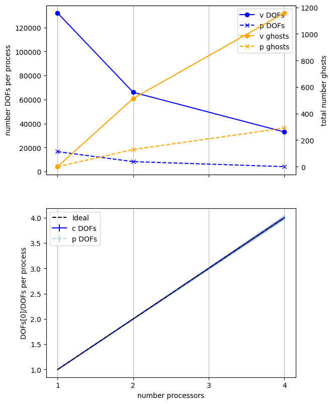
We present a previously computed result using ne = 256, p = 1 and number = 10 in Figure 2.4.4 generated on a dedicated machine with a local conda installation of the software.
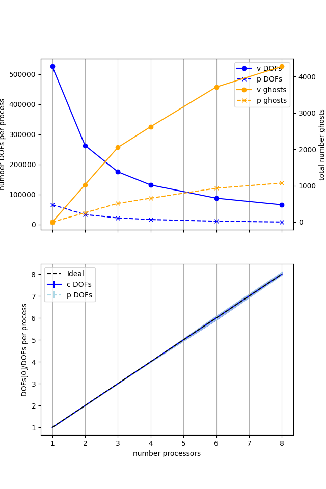
Figure 2.4.4 Numbers of degrees of freedom per process and the total number of ghost degrees of freedom with an increasing number of processes with ne = 256, p = 1 averaged over number = 10 calculations using a local conda installation of the software on a dedicated machine.
Here we can see that the number of degrees of freedom per process is decreasing (with the numbers of DOFs per process scaling ideally) with an increasing number of processes but the total (sum over all processes) of the ghost degrees of freedom is simultaneously increasing. So, while the cost per process is decreasing, the communications cost (as measured by the number of ghost degrees of freedom) is increasing, contributing to scaling not being ideal.
We have already tested that this implementation converges in parallel so we move onto testing if the new implementation scales any better.
Direct (nest)#
We test the new implementation, using a PETSc MATNEST matrix with the same default solver options (plus an additional option to output log information for MUMPS so we can profile it too).
petsc_options = {'ksp_type' : 'preonly', 'pc_type' : 'lu', 'pc_factor_mat_solver_type' : 'mumps', 'mat_mumps_icntl_4': 2}

maxtimes_dn, maxmumpstimes_dn, extradiagout_dn  = fenics_sz.utils.ipp.profile_parallel(nprocs_scale, steps, path, 'fenics_sz.background.batchelor_nest', 'solve_batchelor_nest',
                                                        ne, p, number=number, include_mumps_times=True,
                                                        extra_diagnostics_func=extra_parallel_diagnostics,
                                                        petsc_options=petsc_options,
                                                        output_filename=output_folder / 'batchelor_scaling_direct_nest.png')
maxtimes['Direct (nest)'] = maxtimes_dn
=========================
                     1           2           4
Mesh                 0.026       0.033       0.055
Function spaces      0.017       0.015       0.016
Assemble             0.154       0.098       0.093
Solve                1.496       1.299       1.455
=========================
MUMPS analysis       0.70842     0.71686     0.89063
MUMPS factorization  0.66003     0.4939      0.48233
MUMPS solve          0.04566     0.03097     0.02999
=========================
v_ndofs_max          132098      66160       33208
v_ndofs_min          132098      65938       32728
v_ndofs_sum          132098      132098      132098
v_ndofs_avg          132098      66049       33024.5
v_nghosts_max        0           282         376
v_nghosts_min        0           232         244
v_nghosts_sum        0           514         1158
v_nghosts_avg        0           257         289.5
p_ndofs_max          16641       8329        4190
p_ndofs_min          16641       8312        4128
p_ndofs_sum          16641       16641       16641
p_ndofs_avg          16641       8320.5      4160.25
p_nghosts_max        0           71          94
p_nghosts_min        0           58          63
p_nghosts_sum        0           129         291
p_nghosts_avg        0           64.5        72.75
=========================
***********  profiling figure in output/batchelor_scaling_direct_nest.png
If sufficient computational resources are available when running this notebook (unlikely during website generation) this should show similar results to the original version. For comparison we provide the output of this notebook using ne = 256, p = 1 and number = 10 in Figure 2.4.5 generated on a dedicated machine with a local conda installation of the software.
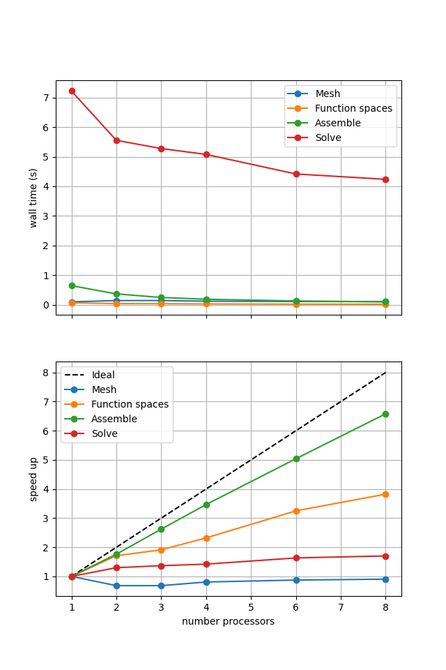
Figure 2.4.5 Scaling results for a direct solver using a MATNEST matrix with ne = 256, p = 1 averaged over number = 10 calculations using a local conda installation of the software on a dedicated machine.
Figure 2.4.5 shows that our new implementation scales in a similar manner to the original when using a direct solver. To double check that it is working we re-run our convergence test in parallel.
# the list of the number of processors to test the convergence on
nprocs_conv = [2,]
# List of polynomial orders to try
ps = [1, 2]
# List of resolutions to try
nelements = [10, 20, 40, 80]
errors_l2_all = fenics_sz.utils.ipp.run_parallel(nprocs_conv, path, 'fenics_sz.background.batchelor_nest', 'convergence_errors_nest', ps, nelements)
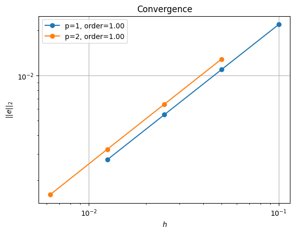
for errors_l2 in errors_l2_all:
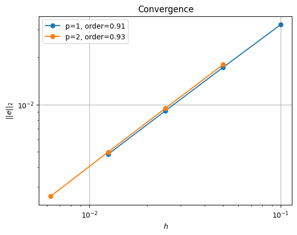
test_passes = test_plot_convergence(ps, nelements, errors_l2)
assert(test_passes)
order of accuracy p=1, order=1.0000050785210868
order of accuracy p=2, order=0.9999999771173882

Which does scale (suboptimally) as expected.
Iterative (nest, refpt)#
Unlike the original implementation, we should be able to use an iterative solver (e.g., minres) on the new implementation. We do this by applying a fieldsplit preconditioner using a pressure mass matrix to precondition the zero saddle point block of the Stokes problem.
petsc_options = {'ksp_type':'minres',
                 'pc_type':'fieldsplit',
                 'pc_fieldsplit_type': 'additive',
                 'fieldsplit_v_ksp_type':'preonly',
                 'fieldsplit_v_pc_type':'gamg',
                 'fieldsplit_v_pc_gamg_threshold_scale' : 1.0,
                 'fieldsplit_v_pc_gamg_threshold' : 0.01,
                 'fieldsplit_v_pc_gamg_coarse_eq_limit' : 800,
                 'fieldsplit_p_ksp_type':'preonly',
                 'fieldsplit_p_pc_type':'jacobi'}

maxtimes['Iterative (nest, refpt)'], _, _ = fenics_sz.utils.ipp.profile_parallel(nprocs_scale, steps, path, 'fenics_sz.background.batchelor_nest', 'solve_batchelor_nest',
                                                        ne, p, number=number, petsc_options=petsc_options,
                                                        output_filename=output_folder / 'batchelor_scaling_iterative_refpt.png')
=========================
                 1           2           4
Mesh             0.024       0.033       0.057
Function spaces  0.02        0.014       0.015
Assemble         0.18        0.111       0.109
Solve            2.78        1.679       1.585
=========================
***********  profiling figure in output/batchelor_scaling_iterative_refpt.png
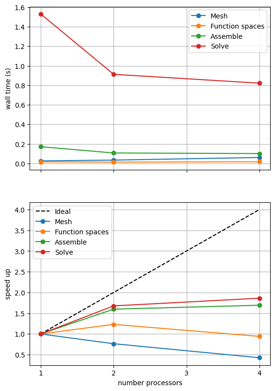
If sufficient computational resources are available when running this notebook (unlikely during website generation) this should show that the scaling (“speed up”) of our solve step has improved but the overall wall time appears larger than when using a direct (LU) solver. For comparison we provide the output of this notebook using ne = 256, p = 1 and number = 10 in Figure 2.4.4 generated on a dedicated machine with a local conda installation of the software.
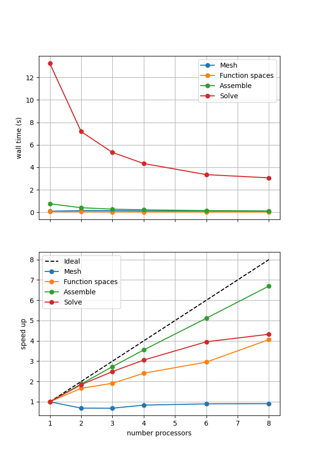
Figure 2.4.4 Scaling results for a direct solver using a MATNEST matrix with ne = 256, p = 1 averaged over number = 10 calculations using a local conda installation of the software on a dedicated machine.
Figure 2.4.4 indeed shows that the scaling (“speed up”) of our solve step has improved but the overall wall time appears larger than when using a direct (LU) solver. As before, we double check our solution is converging in parallel using these solver options.
errors_l2_all = fenics_sz.utils.ipp.run_parallel(nprocs_conv, path, 'fenics_sz.background.batchelor_nest', 'convergence_errors_nest', ps, nelements, petsc_options=petsc_options)

for errors_l2 in errors_l2_all:
    test_passes = test_plot_convergence(ps, nelements, errors_l2)
    assert(test_passes)
order of accuracy p=1, order=1.0003478749723533
order of accuracy p=2, order=1.002984039768499
Iterative (nest, null space)#
Our new implementation also allows us to try another method of dealing with the pressure nullspace - removing the null space at each iteration of the solver rather than imposing a reference point. We can test this method by setting the attach_nullspace flag to True.
petsc_options = {'ksp_type':'minres',
                 'pc_type':'fieldsplit',
                 'pc_fieldsplit_type': 'additive',
                 'fieldsplit_v_ksp_type':'preonly',
                 'fieldsplit_v_pc_type':'gamg',
                 'pc_gamg_threshold_scale' : 1.0,
                 'pc_gamg_threshold' : 0.01,
                 'pc_gamg_coarse_eq_limit' : 800,
                 'fieldsplit_p_ksp_type':'preonly',
                 'fieldsplit_p_pc_type':'jacobi'}

maxtimes['Iterative (nest, ns)'], _, _ = fenics_sz.utils.ipp.profile_parallel(nprocs_scale, steps, path, 'fenics_sz.background.batchelor_nest', 'solve_batchelor_nest',
                                                        ne, p, number=number, petsc_options=petsc_options, attach_nullspace=True,
                                                        output_filename=output_folder / 'batchelor_scaling_iterative_ns.png')
=========================
                 1           2           4
Mesh             0.026       0.034       0.061
Function spaces  0.016       0.013       0.017
Assemble         0.171       0.107       0.101
Solve            1.531       0.913       0.822
=========================
*********** profiling figure in output/batchelor_scaling_iterative_ns.png
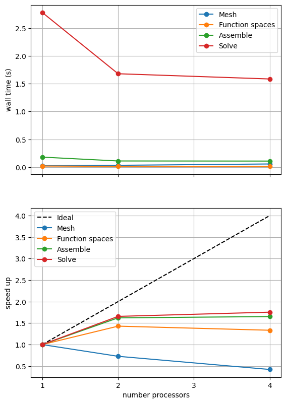
If sufficient computational resources are available when running this notebook (unlikely during website generation) this should show a substantial reduction in the cost of our solution while maintaining reasonable scaling (“speed up”) at this problem size. For comparison we provide the output of this notebook using ne = 256, p = 1 and number = 10 in Figure 2.4.5 generated on a dedicated machine with a local conda installation of the software.
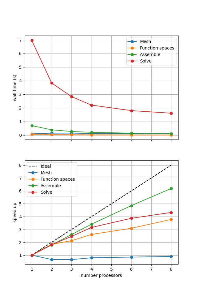
Figure 2.4.5 Scaling results for a direct solver using a MATNEST matrix with ne = 256, p = 1 averaged over number = 10 calculations using a local conda installation of the software on a dedicated machine.
Figure 2.4.5 indeed shows a substantially lower cost while also scaling reasonably well. Again, we double check our solution is converging in parallel using these solver options.
errors_l2_all = fenics_sz.utils.ipp.run_parallel(nprocs_conv, path, 'fenics_sz.background.batchelor_nest', 'convergence_errors_nest', ps, nelements, petsc_options=petsc_options, attach_nullspace=True)

for errors_l2 in errors_l2_all:
    test_passes = test_plot_convergence(ps, nelements, errors_l2)
    assert(test_passes)
order of accuracy p=1, order=0.9126715734780724
order of accuracy p=2, order=0.9274958545683684
We see that we are converging but at a slightly lower rate than using the reference point.
Comparison#
We can more easily compare the different solution method directly by plotting their walltimes for assembly and solution.
# choose which steps to compare
compare_steps = ['Assemble', 'Solve']

# set up a figure for plotting
fig, axs = pl.subplots(nrows=len(compare_steps), figsize=[6.4,4.8*len(compare_steps)], sharex=True)
if len(compare_steps) == 1: axs = [axs]
for i, step in enumerate(compare_steps):
    s = steps.index(step)
    for name, lmaxtimes in maxtimes.items():
        axs[i].plot(nprocs_scale, [t[s] for t in lmaxtimes], 'o-', label=name)
    axs[i].xaxis.set_major_locator(ticker.MaxNLocator(integer=True))
    axs[i].set_title(step)
    axs[i].legend()
    axs[i].set_ylabel('wall time (s)')
    axs[i].grid()
axs[-1].set_xlabel('number processors')
# save the figure
fig.savefig(output_folder / 'batchelor_scaling_comparison.png')
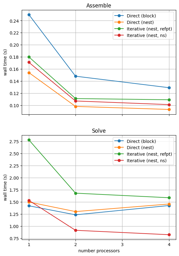
With sufficient computational resources we will see that the MATNEST approach has lowered our assembly costs, though as this is such a small overall part of our wall time it doesn’t make a big impact in this case. However, the decreased cost and improved scaling of the iterative solver method (removing the nullspace iteratively) makes a substantial difference to the cost of our solution. We provide the output of this notebook using ne = 256, p = 1 and number = 10 in Figure 2.4.6 generated on a dedicated machine with a local conda installation of the software.
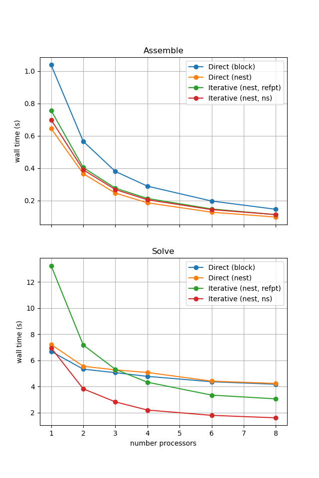
Figure 2.4.6 Comparison of scaling results for different solution strategies with ne = 256, p = 1 averaged over number = 10 calculations using a local conda installation of the software on a dedicated machine.
In the next example we will see how the advantage of using the iterative method is removed at these problem sizes when we have to solve the equations multiple times.