Steady-State Subduction Zone Setup#
Themes and variations - higher resolution#
In this notebook we will try increasing the resolution of the benchmark cases to see if we match the benchmarks better.
Preamble#
Let’s start by adding the path to the modules in the python folder to the system path (so we can find the our custom modules).
import sys, os
basedir = ''
if "__file__" in globals(): basedir = os.path.dirname(__file__)
sys.path.insert(0, os.path.join(basedir, os.path.pardir, os.path.pardir, 'python'))
Then load everything we need from sz_problems and other modules.
import fenics_sz.utils
from fenics_sz.sz_problems.sz_params import default_params, allsz_params
from fenics_sz.sz_problems.sz_slab import create_slab
from fenics_sz.sz_problems.sz_geometry import create_sz_geometry
from fenics_sz.sz_problems.sz_steady_isoviscous import SteadyIsoSubductionProblem
from fenics_sz.sz_problems.sz_steady_dislcreep import SteadyDislSubductionProblem
import pathlib
output_folder = pathlib.Path(os.path.join(basedir, "output"))
output_folder.mkdir(exist_ok=True, parents=True)
Benchmark case 1#
xs = [0.0, 140.0, 240.0, 400.0]
ys = [0.0, -70.0, -120.0, -200.0]
lc_depth = 40
uc_depth = 15
coast_distance = 0
extra_width = 0
sztype = 'continental'
io_depth_1 = 139
A      = 100.0      # age of subducting slab (Myr)
qs     = 0.065      # surface heat flux (W/m^2)
Vs     = 100.0      # slab speed (mm/yr)
resscale2 = 2.5
slab_resscale2 = create_slab(xs, ys, resscale2, lc_depth)
geom_resscale2 = create_sz_geometry(slab_resscale2, resscale2, sztype, io_depth_1, extra_width,
                           coast_distance, lc_depth, uc_depth)
sz_case1_resscale2 = SteadyIsoSubductionProblem(geom_resscale2, A=A, Vs=Vs, sztype=sztype, qs=qs)
print("\nSolving steady state flow with isoviscous rheology...")
sz_case1_resscale2.solve()
Solving steady state flow with isoviscous rheology...
diag_resscale2 = sz_case1_resscale2.get_diagnostics()

print('')
print('{:<12} {:<12} {:<12} {:<12} {:<12} {:<12}'.format('resscale', 'T_ndof', 'T_{200,-100}', 'Tbar_s', 'Tbar_w', 'Vrmsw'))
print('{:<12.4g} {:<12d} {:<12.4f} {:<12.4f} {:<12.4f} {:<12.4f}'.format(resscale2, *diag_resscale2.values()))
resscale     T_ndof       T_{200,-100} Tbar_s       Tbar_w       Vrmsw
2.5          21229        516.9912     451.7434     926.4091     34.6378
For comparison here are the values reported for case 1 using TerraFERMA in Wilson & van Keken, 2023:
|
\(T_{\text{ndof}} \) |
\(T_{(200,-100)}^*\) |
\(\overline{T}_s^*\) |
\( \overline{T}_w^* \) |
\(V_{\text{rms},w}^*\) |
|---|---|---|---|---|---|
2.0 |
21403 |
517.17 |
451.83 |
926.62 |
34.64 |
1.0 |
83935 |
516.95 |
451.71 |
926.33 |
34.64 |
0.5 |
332307 |
516.86 |
451.63 |
926.15 |
34.64 |
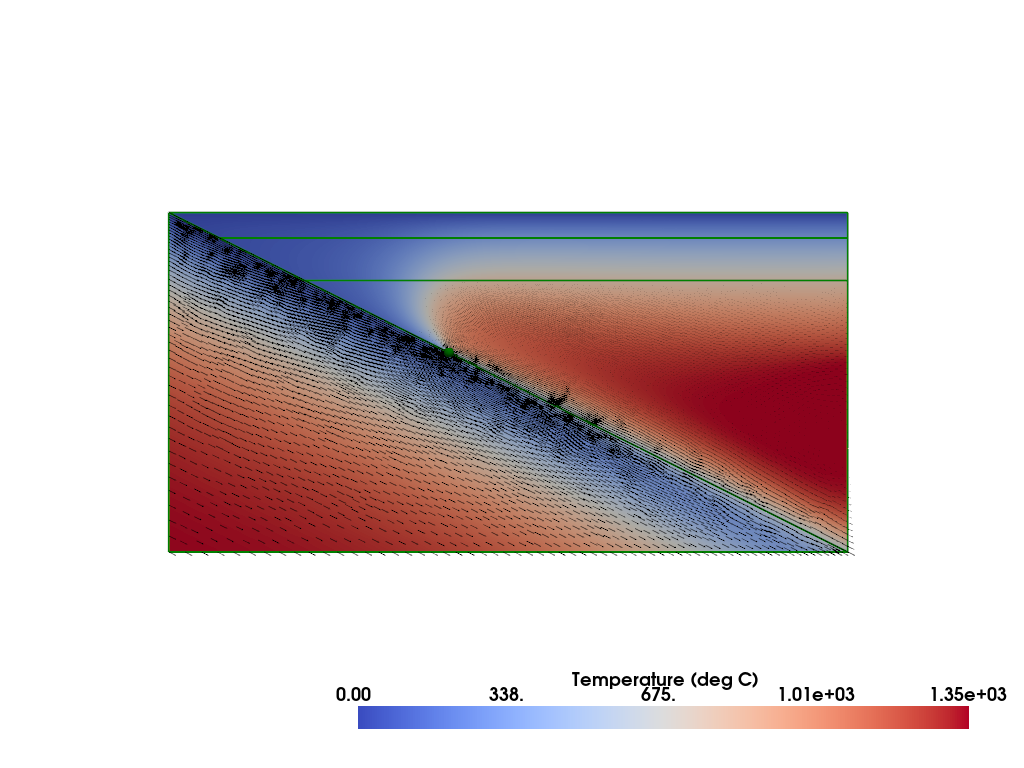
plotter_case1_resscale2 = fenics_sz.utils.plot.plot_scalar(sz_case1_resscale2.T_i, scale=sz_case1_resscale2.T0, gather=True, cmap='coolwarm', scalar_bar_args={'title': 'Temperature (deg C)', 'bold':True})
fenics_sz.utils.plot.plot_vector_glyphs(sz_case1_resscale2.vw_i, plotter=plotter_case1_resscale2, gather=True, factor=0.05, color='k', scale=fenics_sz.utils.mps_to_mmpyr(sz_case1_resscale2.v0))
fenics_sz.utils.plot.plot_vector_glyphs(sz_case1_resscale2.vs_i, plotter=plotter_case1_resscale2, gather=True, factor=0.05, color='k', scale=fenics_sz.utils.mps_to_mmpyr(sz_case1_resscale2.v0))
sz_case1_resscale2.geom.pyvistaplot(plotter=plotter_case1_resscale2, color='green', width=2)
cdpt = sz_case1_resscale2.geom.slab_spline.findpoint('Slab::FullCouplingDepth')
fenics_sz.utils.plot.plot_points([[cdpt.x, cdpt.y, 0.0]], plotter=plotter_case1_resscale2, render_points_as_spheres=True, point_size=10.0, color='green')
fenics_sz.utils.plot.plot_show(plotter_case1_resscale2)
fenics_sz.utils.plot.plot_save(plotter_case1_resscale2, output_folder / "sz_steady_tests_case1_resscale2_solution.png")
# clean up
del plotter_case1_resscale2
del sz_case1_resscale2
del geom_resscale2
Benchmark case 2#
io_depth_2 = 154.0
geom_case2_resscale2 = create_sz_geometry(slab_resscale2, resscale2, sztype, io_depth_2, extra_width,
                                          coast_distance, lc_depth, uc_depth)
sz_case2_resscale2 = SteadyDislSubductionProblem(geom_case2_resscale2, A=A, Vs=Vs, sztype=sztype, qs=qs)
print("\nSolving steady state flow with dislocation creep rheology...")
sz_case2_resscale2.solve()
Solving steady state flow with dislocation creep rheology...
Iteration   Residual     Relative Residual
------------------------------------------
0           13486        1
1           2514.09      0.186423
2           350.886      0.0260186
3           129.152      0.00957675
4           57.9183      0.00429471
5           31.7142      0.00235165
6           19.3757      0.00143673
7           12.787       0.00094817
8           8.96835      0.000665013
9           6.51475      0.000483076
10          4.85702      0.000360153
11          3.67984      0.000272864
12          2.81527      0.000208755
13          2.16655      0.000160652
14          1.67301      0.000124056
15          1.29409      9.5958e-05
16          1.00144      7.42577e-05
17          0.774535     5.74326e-05
18          0.598143     4.4353e-05
19          0.460808     3.41694e-05
20          0.353827     2.62367e-05
21          0.270542     2.0061e-05
22          0.205829     1.52624e-05
23          0.155716     1.15465e-05
24          0.117107     8.68359e-06
25          0.0875775    6.49397e-06
26          0.0652259    4.83657e-06
diag_case2_resscale2 = sz_case2_resscale2.get_diagnostics()

print('')
print('{:<12} {:<12} {:<12} {:<12} {:<12} {:<12}'.format('resscale', 'T_ndof', 'T_{200,-100}', 'Tbar_s', 'Tbar_w', 'Vrmsw'))
print('{:<12.4g} {:<12d} {:<12.4f} {:<12.4f} {:<12.4f} {:<12.4f}'.format(resscale2, *diag_case2_resscale2.values()))
resscale     T_ndof       T_{200,-100} Tbar_s       Tbar_w       Vrmsw
2.5          21281        683.6152     572.9186     934.6403     40.8429
For comparison here are the values reported for case 2 using TerraFERMA in Wilson & van Keken, 2023:
|
\(T_{\text{ndof}} \) |
\(T_{(200,-100)}^*\) |
\(\overline{T}_s^*\) |
\( \overline{T}_w^* \) |
\(V_{\text{rms},w}^*\) |
|---|---|---|---|---|---|
2.0 |
21403 |
683.05 |
571.58 |
936.65 |
40.89 |
1.0 |
83935 |
682.87 |
572.23 |
936.11 |
40.78 |
0.5 |
332307 |
682.80 |
572.05 |
937.37 |
40.77 |
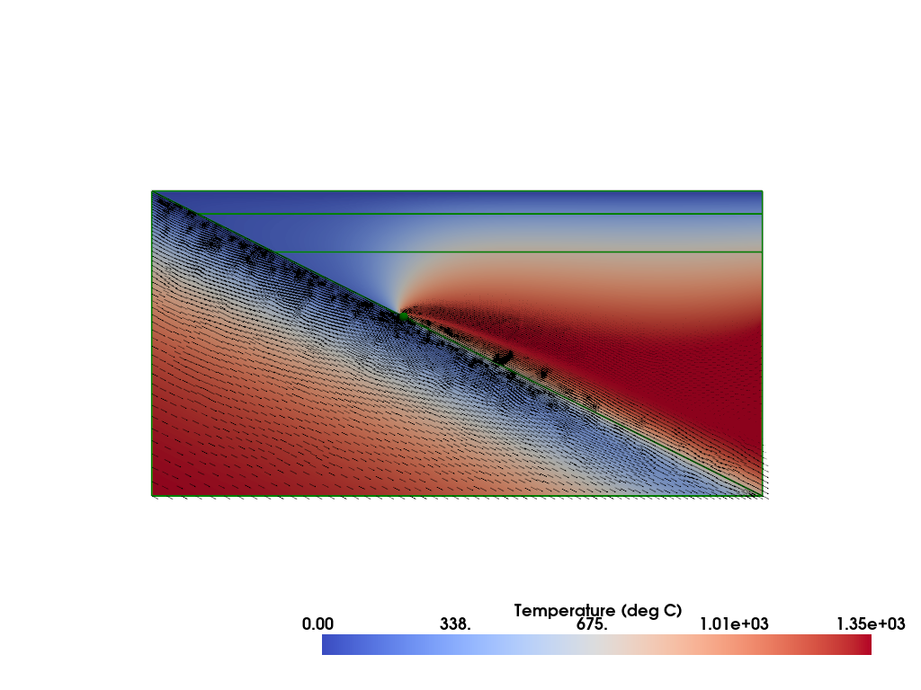
plotter_case2_resscale2 = fenics_sz.utils.plot.plot_scalar(sz_case2_resscale2.T_i, scale=sz_case2_resscale2.T0, gather=True, cmap='coolwarm', scalar_bar_args={'title': 'Temperature (deg C)', 'bold':True})
fenics_sz.utils.plot.plot_vector_glyphs(sz_case2_resscale2.vw_i, plotter=plotter_case2_resscale2, gather=True, factor=0.05, color='k', scale=fenics_sz.utils.mps_to_mmpyr(sz_case2_resscale2.v0))
fenics_sz.utils.plot.plot_vector_glyphs(sz_case2_resscale2.vs_i, plotter=plotter_case2_resscale2, gather=True, factor=0.05, color='k', scale=fenics_sz.utils.mps_to_mmpyr(sz_case2_resscale2.v0))
sz_case2_resscale2.geom.pyvistaplot(plotter=plotter_case2_resscale2, color='green', width=2)
cdpt = sz_case2_resscale2.geom.slab_spline.findpoint('Slab::FullCouplingDepth')
fenics_sz.utils.plot.plot_points([[cdpt.x, cdpt.y, 0.0]], plotter=plotter_case2_resscale2, render_points_as_spheres=True, point_size=10.0, color='green')
fenics_sz.utils.plot.plot_show(plotter_case2_resscale2)
fenics_sz.utils.plot.plot_save(plotter_case2_resscale2, output_folder / "sz_steady_tests_case2_resscale2_solution.png")
# clean up
del plotter_case2_resscale2
del sz_case2_resscale2
del geom_case2_resscale2
del slab_resscale2
In the next notebook we will try seeing the effect of varying the coupling depth.