Poisson Example 2D#
A specific example#
In this case we use a manufactured solution (that is, one that is not necessarily an example of a solution to a PDE representing a naturally occurring physical problem) where we take a known analytical solution \(T(x,y)\) and substitute this into the original equation to find \(h\), then use this as the right-hand side in our numerical test. We choose \(T(x,y) = \exp\left(x+\tfrac{y}{2}\right)\), which is the solution to
Solving the Poisson equation numerically in a unit square, \(\Omega=[0,1]\times[0,1]\), for the approximate solution \(\tilde{T} \approx T\), we impose the boundary conditions
representing an essential Dirichlet condition on the value of \(\tilde{T}\) and natural Neumann conditions on \(\nabla\tilde{T}\).
Implementation#
This example was presented by Wilson & van Keken, 2023 using FEniCS v2019.1.0 and TerraFERMA, a GUI-based model building framework that also uses FEniCS v2019.1.0. Here we reproduce these results using the latest version of FEniCS, FEniCSx.
Preamble#
We start by loading all the modules we will require.
from mpi4py import MPI
import dolfinx as df
from petsc4py import PETSc
import dolfinx.fem.petsc
import numpy as np
import ufl
import matplotlib.pyplot as pl
import sys, os
basedir = ''
if "__file__" in globals(): basedir = os.path.dirname(__file__)
sys.path.insert(0, os.path.join(basedir, os.path.pardir, os.path.pardir, 'python'))
import fenics_sz.utils.plot
import pathlib
output_folder = pathlib.Path(os.path.join(basedir, "output"))
output_folder.mkdir(exist_ok=True, parents=True)
Solution#
We then declare a python function solve_poisson_2d that contains a complete description of the discrete Poisson equation problem.
This function follows much the same flow as described in the introduction
we describe the unit square domain \(\Omega = [0,1]\times[0,1]\) and discretize it into \(2 \times\)
ne\(\times\)netriangular elements or cells to make ameshwe declare the function space,
V, to use Lagrange polynomials of degreepwe define the Dirichlet boundary condition,
bcat the boundaries where \(x=0\) or \(y=0\), setting the desired value there to the known exact solutionwe define a finite element function,
gN, containing the values of \(\nabla \tilde{T}\) on the Neumann boundaries where \(x=1\) or \(y=1\) (note that because this is a natural boundary condition it will be used in the weak form rather than as a boundary condition object)we define the right hand side forcing function \(h\),
husing the function space we declare trial,
T_a, and test,T_t, functions and use them to describe the discrete weak forms,Sandf, that will be used to assemble a left-hand-side matrix \(\mathbf{S}_m\) (Sm) and right-hand-side vector \(\mathbf{f}_m\) (fm)we assemble the matrix problem and solve it using a PETSc linear algebra back-end, return the solution temperature,
T_i
Note that to aid with profiling in subsequent notebooks, in a departure from the implementation for the 1D case, we
allow solver options to be passed into the function in a
petsc_optionsdictionarygroup some of the steps together in timed blocks
split the single solution step using
LinearProbleminto assembly and solution steps to time each independently
For a more detailed description of solving the Poisson equation using FEniCSx, see the FEniCSx tutorial.
def solve_poisson_2d(ne, p=1, petsc_options=None):
    """
    A python function to solve a two-dimensional Poisson problem
    on a unit square domain.
    Parameters:
    * ne - number of elements in each dimension
    * p  - polynomial order of the solution function space
    * petsc_options - a dictionary of petsc options to pass to the solver
                      (defaults to an LU direct solver using the MUMPS library)
    """

    # Set the default PETSc solver options if none have been supplied
    if petsc_options is None:
        petsc_options = {"ksp_type": "preonly", \
                         "pc_type": "lu",
                         "pc_factor_mat_solver_type": "mumps"}
    opts = PETSc.Options()
    for k, v in petsc_options.items(): opts[k] = v

    # Describe the domain (a unit square)
    # and also the tessellation of that domain into ne
    # equally spaced squares in each dimension which are
    # subdivided into two triangular elements each
    with df.common.Timer("Mesh"):
        mesh = df.mesh.create_unit_square(MPI.COMM_WORLD, ne, ne, ghost_mode=df.mesh.GhostMode.none)

    # Define the solution function space using Lagrange polynomials
    # of order p
    with df.common.Timer("Function spaces"):
        V = df.fem.functionspace(mesh, ("Lagrange", p))

    with df.common.Timer("Dirichlet BCs"):
        # Define the location of the boundary condition, x=0 and y=0
        def boundary(x):
            return np.logical_or(np.isclose(x[0], 0), np.isclose(x[1], 0))
        boundary_dofs = df.fem.locate_dofs_geometrical(V, boundary)
        # Specify the value and define a Dirichlet boundary condition (bc)
        gD = df.fem.Function(V)
        gD.interpolate(lambda x: np.exp(x[0] + x[1]/2.))
        bc = df.fem.dirichletbc(gD, boundary_dofs)

    with df.common.Timer("Neumann BCs"):
        # Get the coordinates
        x = ufl.SpatialCoordinate(mesh)
        # Define the Neumann boundary condition function
        gN = ufl.as_vector((ufl.exp(x[0] + x[1]/2.), 0.5*ufl.exp(x[0] + x[1]/2.)))
        # Define the right hand side function, h
        h = -5./4.*ufl.exp(x[0] + x[1]/2.)

    with df.common.Timer("Forms"):
        T_a = ufl.TrialFunction(V)
        T_t = ufl.TestFunction(V)
        # Get the unit vector normal to the facets
        n = ufl.FacetNormal(mesh)
        # Define the integral to be assembled into the stiffness matrix
        S = df.fem.form(ufl.inner(ufl.grad(T_t), ufl.grad(T_a))*ufl.dx)
        # Define the integral to be assembled into the forcing vector,
        # incorporating the Neumann boundary condition weakly
        f = df.fem.form(T_t*h*ufl.dx + T_t*ufl.inner(gN, n)*ufl.ds)

    # The next two sections "Assemble" and "Solve"
    # are the equivalent of the much simpler:
    # ```
    # problem = df.fem.petsc.LinearProblem(S, f, bcs=[bc], \
    #                                      petsc_options=petsc_options)
    # T_i = problem.solve()
    # ```
    # We split them up here so we can time and profile each step separately.
    with df.common.Timer("Assemble"):
        # Assemble the matrix from the S form
        Sm = df.fem.petsc.assemble_matrix(S, bcs=[bc])
        Sm.assemble()
        # Assemble the R.H.S. vector from the f form
        fm = df.fem.petsc.assemble_vector(f)

        # Set the boundary conditions
        df.fem.petsc.apply_lifting(fm, [S], bcs=[[bc]])
        fm.ghostUpdate(addv=PETSc.InsertMode.ADD, mode=PETSc.ScatterMode.REVERSE)
        df.fem.petsc.set_bc(fm, [bc])

    with df.common.Timer("Solve"):
        # Setup the solver (a PETSc KSP object)
        solver = PETSc.KSP().create(MPI.COMM_WORLD)
        solver.setOperators(Sm)
        solver.setFromOptions()

        # Set up the solution function
        T_i = df.fem.Function(V)
        # Call the solver
        solver.solve(fm, T_i.x.petsc_vec)
        # Communicate the solution across processes
        T_i.x.scatter_forward()

    with df.common.Timer("Cleanup"):
        solver.destroy()
        Sm.destroy()
        fm.destroy()

    return T_i
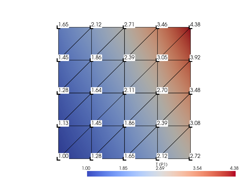
We can now numerically solve the equations using, e.g., 4 elements and piecewise linear polynomials.
ne = 4
p = 1
T_P1 = solve_poisson_2d(ne, p=p)
T_P1.name = "T (P1)"
And use some utility functions (see python/fenics_sz/utils/plot.py) to plot it.
# plot the solution as a colormap
plotter_P1 = fenics_sz.utils.plot.plot_scalar(T_P1, gather=True, cmap='coolwarm')
# plot the mesh
fenics_sz.utils.plot.plot_mesh(T_P1.function_space.mesh, plotter=plotter_P1, gather=True, show_edges=True, style="wireframe", color='k', line_width=2)
# plot the values of the solution at the nodal points
fenics_sz.utils.plot.plot_scalar_values(T_P1, plotter=plotter_P1, gather=True, point_size=15, font_size=22, shape_color='w', text_color='k', bold=False)
# show the plot
fenics_sz.utils.plot.plot_show(plotter_P1)
# save the plot
fenics_sz.utils.plot.plot_save(plotter_P1, output_folder / "2d_poisson_P1_solution.png")
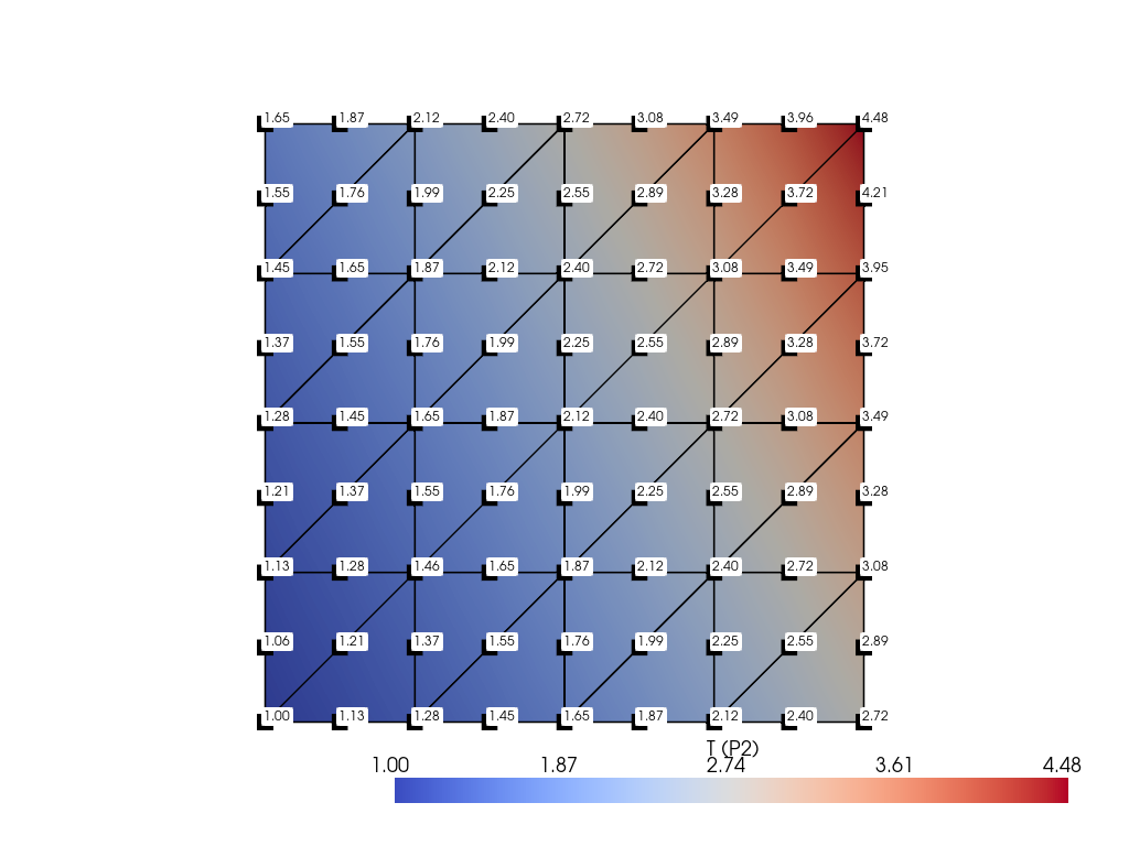
Similarly, we can solve the equation using quadratic elements (p=2).
ne = 4
p = 2
T_P2 = solve_poisson_2d(ne, p=p)
T_P2.name = "T (P2)"
# plot the solution as a colormap
plotter_P2 = fenics_sz.utils.plot.plot_scalar(T_P2, gather=True, cmap='coolwarm')
# plot the mesh
fenics_sz.utils.plot.plot_mesh(T_P2.function_space.mesh, plotter=plotter_P2, gather=True, show_edges=True, style="wireframe", color='k', line_width=2)
# plot the values of the solution at the nodal points
fenics_sz.utils.plot.plot_scalar_values(T_P2, plotter=plotter_P2, gather=True, point_size=15, font_size=12, shape_color='w', text_color='k', bold=False)
# show the plot
fenics_sz.utils.plot.plot_show(plotter_P2)
# save the plot
fenics_sz.utils.plot.plot_save(plotter_P2, output_folder / "2d_poisson_P2_solution.png")
Themes and variations#
The solution above looks qualitatively good but it is always essential to test our implementation. Using the 1D problem as an example users are encouraged to try the following interactive tasks.
Given that we know the exact solution to this problem is \(T(x,y) = \exp\left(x+\tfrac{y}{2}\right)\) write a python function to evaluate the error in our numerical solution.
Loop over a variety of
nes andps and check that the numerical solution converges with an increasing number of degrees of freedom.
Finally,
To try writing your own weak form, write an equation for the gradient of \(\tilde{T}\), describe it using ufl, solve it, and plot the solution.
We will provide solutions to these tasks in the next notebook.