Subduction Zone Model Setup#
Implementation#
As a reminder our implementation is following a similar workflow to that seen in the background examples.
we will describe the subduction zone geometry and tesselate it into non-overlapping triangles to create a mesh
we will declare function spaces for the temperature, wedge velocity and pressure, and slab velocity and pressure
using these function spaces we will declare trial and test functions
we will define Dirichlet boundary conditions at the boundaries as described in the introduction
we will describe discrete weak forms for temperature and each of the coupled velocity-pressure systems that will be used to assemble the matrices (and vectors) to be solved
we will set up matrices and solvers for the discrete systems of equations
we will solve the matrix problems
In the previous three notebooks we have only tackled steps 1-4. We now move onto steps 5-7, implementing the Stokes weak forms that are common across all the problems we want to tackle, setting up the resulting matrix-vector system and solving it. We do this by deriving a SubductionProblem class from the base BaseSubductionProblem class we implemented in notebooks/03_sz_problems/3.2d_sz_base.ipynb. We also implement two extra classes StokesSolverNest and TemperatureSolver to handle the assembly and solution of our matrix-vector systems in this notebook.
Preamble#
Let’s start by adding the path to the modules in the python folder to the system path (so we can find the our custom modules).
import sys, os
basedir = ''
if "__file__" in globals(): basedir = os.path.dirname(__file__)
sys.path.insert(0, os.path.join(basedir, os.path.pardir, os.path.pardir, 'python'))
Let’s also load the module generated by the previous notebooks to get access to the parameters and functions defined there.
from fenics_sz.sz_problems.sz_params import default_params, allsz_params
from fenics_sz.sz_problems.sz_slab import create_slab
from fenics_sz.sz_problems.sz_geometry import create_sz_geometry
from fenics_sz.sz_problems.sz_base import BaseSubductionProblem
Then let’s load all the required modules at the beginning.
import fenics_sz.geometry as geo
import fenics_sz.utils
from mpi4py import MPI
import dolfinx as df
import dolfinx.fem.petsc
from petsc4py import PETSc
import numpy as np
import scipy as sp
import ufl
import basix.ufl as bu
import matplotlib.pyplot as pl
import copy
import pyvista as pv
import pathlib
output_folder = pathlib.Path(os.path.join(basedir, "output"))
output_folder.mkdir(exist_ok=True, parents=True)
SubductionProblem class#
We continue building on the BaseSubductionProblem class implemented in notebooks/03_sz_problems/3.2d_sz_base.ipynb, deriving a SubductionProblem class that includes (some) equations and solution algorithms.
5. Equations#
In all our problems we wish to solve the Stokes equations for the velocity \(\vec{v}\), and pressure, \(p\)
for an incompressible viscous fluid where \(\vec{v}\) can be the wedge velocity, \(\vec{v}_w\) (wedge_vw_i), or the slab velocity \(\vec{v}_s\) (slab_vs_i), and similarly \(p\) can be the wedge pressure, \(p_w\) (wedge_pw_i), or the slab pressure \(p_s\) (slab_ps_i). \(\eta\) is the non-dimensional viscosity.
Our goal is to discretize this system of equations using finite elements such that we have systems like
where \(S_s = S_s(u_{s_t}, u_{s_a})\) is a bilinear form of the combined velocity-pressure test \(u_{s_t}\) and trial \(u_{s_a}\) functions that will be used to assemble a left-hand side matrix and \(f_s = f_s(u_{s_t})\) is a linear form that will be used to describe a right-hand side vector in a matrix-vector equation for the velocity-pressure solution \(u_s = \left(\vec{v}, p\right)^T\).
To get this form we multiply the Stokes equations by the test function \(u_t = \left(\vec{v}_{w_t}, p_{w_t}\right)^T\), integrate by parts, and apply appropriate boundary conditions to the resulting boundary integrals (in this case we can just drop them all since all our natural boundary conditions are homogeneous, e.g. equal to 0).
Doing this in the wedge (using the subscript \(w\)) we get
where
and similarly in the slab (using the subscript \(s\)) we get
where
We describe a generalized (not specific to the slab or the wedge) version of these forms in the function stokes_forms and add it to our SubductionProblem class (newly derived from the BaseSubductionProblem class).
class SubductionProblem(BaseSubductionProblem):
    def stokes_forms(self, v_t, p_t, v_a, p_a, v, p, eta=1):
        """
        Return the forms Ss and fs for the matrix problem Ss*us = fs for the Stokes problems
        given the test and trial functions and the mesh.

        Arguments:
          * v_t  - velocity test function
          * p_t  - pressure test function
          * v_a  - velocity trial function
          * p_a  - pressure trial function
          * v    - velocity function
          * p    - pressure function

        Keyword Arguments:
          * eta  - viscosity (optional, defaults to 1 for isoviscous)

        Returns:
          * Ss - lhs bilinear form for the Stokes problem
          * fs - rhs linear form for the Stokes problem
          * rs - residual linear form for the Stokes problem
          * Ms - viscosity weighted pressure bilinear form (preconditioner)
        """
        with df.common.Timer("Forms Stokes"):
            mesh = p.function_space.mesh
            # the stiffness block
            Ks = ufl.inner(ufl.sym(ufl.grad(v_t)), 2*eta*ufl.sym(ufl.grad(v_a)))*ufl.dx
            # gradient of pressure
            Gs = -ufl.div(v_t)*p_a*ufl.dx
            # divergence of velcoity
            Ds = -p_t*ufl.div(v_a)*ufl.dx
            # combined matrix form
            Ss = [[Ks, Gs], [Ds, None]]
            # this problem has no rhs so create a dummy form by multiplying by a zero constant
            zero_v = df.fem.Constant(mesh, df.default_scalar_type((0.0,0.0)))
            zero_p = df.fem.Constant(mesh, df.default_scalar_type(0.0))
            fs = [ufl.inner(v_t, zero_v)*ufl.dx, p_t*zero_p*ufl.dx]
            # residual form
            rs = [ufl.action(Ss[0][0], v) + ufl.action(Ss[0][1], p) - fs[0],
                  ufl.action(Ss[1][0], v) - fs[1]]
            # viscosity weighted pressure mass matrix
            Ms = (p_t*p_a/eta)*ufl.dx
        # return the forms
        return df.fem.form(Ss), df.fem.form(fs), df.fem.form(rs), df.fem.form(Ms)
stokes_forms accepts the viscosity as one of its parameters, defaulting to 1 when the rheology is isoviscous, as in case 1 of the benchmark. For case 2 (and in the global suite) the viscosity is a function of temperature and strain rate following a simplified creep law for dislocation creep in dry olivine from Karato & Wu, 1993
where \(A_\eta^*\) is a prefactor, \(E^*\) is the activation energy, \(R^*\) is the gas constant, \(n\) is a powerlaw index, \(T^*_a\) a linear approximation of an adiabatic temperature using a gradient of 0.3\(^\circ\)C/km with \(T^*_a=0\) at the top of the model (beyond the benchmark this may not be at \(z^*\)=0 due to assumptions of ocean bathymetry) and \(\dot{\epsilon}_{II}^*\) is the second invariant of the deviatoric strain-rate tensor (also known as the effective deviatoric strain rate)
and depends on whether we are in the wedge, where \(\vec{v}^* = \vec{v}_w^*\) is the dimensional wedge velocity, or in the slab, where \(\vec{v}^* = \vec{v}_s^*\) is the dimensional slab velocity.
Since the dynamical range of the viscosity is large over the temperature contrast across subduction zones the viscosity is capped at some arbitrary maximum \(\eta^*_\text{max}\) so that in the variable viscosity case
where \(\eta_0\) is a reference viscosity scale used to non-dimensionalize the viscosity.
We describe this viscosity law in the python function etadisl and allow it to be examined by projecting its values to a finite element function in project_dislocationcreep_viscosity. These are added to the SubductionProblem class below.
class SubductionProblem(SubductionProblem):
    def etadisl(self, v_i, T_i):
        """
        Return a dislocation creep viscosity given a velocity and temperature

        Arguments:
          * v_i - velocity Function
          * T_i - temperature Function

        Returns:
          * eta - viscosity ufl description
        """

        # get the mesh
        mesh = v_i.function_space.mesh
        x = ufl.SpatialCoordinate(mesh)
        zero_c = df.fem.Constant(mesh, df.default_scalar_type(0.0))
        deltaztrench_c = df.fem.Constant(mesh, df.default_scalar_type(self.deltaztrench))
        deltazsurface = ufl.operators.MinValue(ufl.operators.MaxValue(self.deltaztrench*(1. - x[0]/max(self.deltaxcoast, np.finfo(df.default_scalar_type).eps)), zero_c), deltaztrench_c)
        z = -(x[1]+deltazsurface)

        # dimensional temperature in Kelvin with an adiabat added
        Tdim = fenics_sz.utils.nondim_to_K(T_i) + 0.3*z

        # we declare some of the coefficients as dolfinx Constants to prevent the form compiler from
        # optimizing them out of the code due to their small (dimensional) values
        E_c          = df.fem.Constant(mesh, df.default_scalar_type(self.E))
        invetamax_c  = df.fem.Constant(mesh, df.default_scalar_type(self.eta0/self.etamax))
        neII         = (self.nsigma-1.0)/self.nsigma
        invetafact_c = df.fem.Constant(mesh, df.default_scalar_type(self.eta0*(self.e0**neII)/self.Aeta))
        neII_c       = df.fem.Constant(mesh, df.default_scalar_type(neII))

        # strain rate
        edot = ufl.sym(ufl.grad(v_i))
        eII  = ufl.sqrt(0.5*ufl.inner(edot, edot))
        # inverse dimensionless dislocation creep viscosity
        invetadisl = invetafact_c*ufl.exp(-E_c/(self.nsigma*self.R*Tdim))*(eII**neII_c)
        # inverse dimensionless effective viscosity
        inveta = invetadisl + invetamax_c
        # "harmonic mean" viscosity (actually twice the harmonic mean)
        return 1./inveta

    def project_dislocationcreep_viscosity(self, p_eta=0, petsc_options=None):
        """
        Project the dislocation creep viscosity to a function space.

        Keyword Arguments:
          * p_eta         - finite element degree of viscosity function (defaults to 0)
          * petsc_options - a dictionary of petsc options to pass to the solver (defaults to mumps)

        Returns:
          * eta_i - the viscosity Function
        """
        if petsc_options is None:
            petsc_options={"ksp_type": "preonly",
                           "pc_type" : "lu",
                           "pc_factor_mat_solver_type" : "mumps"}
        # set up the functionspace
        V_eta = df.fem.functionspace(self.mesh, ("DG", p_eta))
        # declare the domain wide Function
        eta_i = df.fem.Function(V_eta)
        eta_i.name = "eta"
        # set it to etamax everywhere (will get overwritten)
        eta_i.x.array[:] = self.etamax/self.eta0

        def solve_viscosity(v_i, T_i):
            """
            Solve for the viscosity in subdomains and interpolate it to the parent Function
            """
            mesh = T_i.function_space.mesh
            V_eta = df.fem.functionspace(mesh, ("DG", p_eta))
            eta_a = ufl.TrialFunction(V_eta)
            eta_t = ufl.TestFunction(V_eta)
            Seta = eta_t*eta_a*ufl.dx
            feta = eta_t*self.etadisl(v_i, T_i)*ufl.dx
            problem = df.fem.petsc.LinearProblem(Seta, feta, petsc_options=petsc_options)
            return problem.solve()

        # solve in the wedge
        if self.wedge_rank:
            leta_i = solve_viscosity(self.wedge_vw_i, self.wedge_T_i)
            eta_i.interpolate(leta_i, cells0=np.arange(len(self.wedge_cell_map)),
                              cells1=self.wedge_cell_map)
        # solve in the slab
        if self.slab_rank:
            leta_i = solve_viscosity(self.slab_vs_i, self.slab_T_i)
            eta_i.interpolate(leta_i, cells0=np.arange(len(self.slab_cell_map)),
                              cells1=self.slab_cell_map)

        # wait for all ranks to catch up
        # (some may not have done anything above and
        # letting them carry on messes with profiling)
        self.comm.barrier()

        # return the viscosity
        return eta_i
The forms for the temperature equations will vary depending on if we are solving a steady-state or isoviscous problem so, in this generic class, we will not implement them, instead raising an error if they are requested.
class SubductionProblem(SubductionProblem):
    def temperature_forms(self):
        raise NotImplementedError("temperature_forms not implemented in SubductionProblem")
6. Matrix-Vector System#
With the forms in place (at least for the Stokes problem) we need to assemble them into a matrix-vector system and solve the resulting discrete problem. We use what we learned in the background examples (specifically the Poisson, Batchelor and Blankenbach scaling experiments) and use PETSc MATNEST matrices for assembly and a PETSc KSP solver to solve the resulting matrix-vector system. This combination gives us the most flexibility in solver choice, particularly for the Stokes system.
We set up a python class StokesSolverNest that encapsulates the MATNEST implementation from the Batchelor example to handle assembly and solution of the Stokes system.
class StokesSolverNest:
    def __init__(self, S, f, bcs, v, p, M=None, isoviscous=False, petsc_options=None):
        """
        A python class to create a matrix and a vector for the given Stokes forms and solve the resulting matrix-vector equations.
        Parameters:
          * S   - Stokes bilinear form
          * f   - Stokes RHS linear form
          * bcs - list of Stokes boundary conditions
          * v   - velocity function
          * p   - pressure function
          * M   - viscosity weighted pressure mass matrix bilinear form (defaults to None)
          * isoviscous - if isoviscous assemble the velocity/pressure mass block at setup
                         (defaults to False)
          * petsc_options - a dictionary of petsc options to pass to the Stokes solver
                            (defaults to an LU direct solver using the MUMPS library)
        """
        # Set the default PETSc solver options if none have been supplied
        opts = PETSc.Options()
        if petsc_options is None:
            petsc_options={"ksp_type": "preonly",
                           "pc_type" : "lu",
                           "pc_factor_mat_solver_type" : "mumps"}
        self.prefix = f"stokes_{id(self)}_"
        opts.prefixPush(self.prefix)
        for key, val in petsc_options.items(): opts[key] = val
        opts.prefixPop()

        self.S   = S
        self.f   = f
        self.bcs = bcs
        self.v   = v
        self.p   = p
        self.M   = M
        self.isoviscous = isoviscous

        self.setup_matrices()
        self.setup_solver()

        self.assembled = False

    def __del__(self):
        self.solver.destroy()
        self.Sm.destroy()
        if self.Pm is not None: self.Pm.destroy()
        self.fm.destroy()
        self.x.destroy()

    def setup_matrices(self):
        """
        Setup the matrices for a Stokes problem.
        """
        # retrieve the petsc options
        opts = PETSc.Options()
        pc_type = opts.getString(self.prefix+'pc_type')

        with df.common.Timer("Assemble Stokes"):
            # create the matrix
            self.Sm = df.fem.petsc.create_matrix_nest(self.S)
            # set a flag to indicate that the velocity block is
            # symmetric positive definite (SPD)
            Sm00 = self.Sm.getNestSubMatrix(0, 0)
            Sm00.setOption(PETSc.Mat.Option.SPD, True)

            # assemble the pre-conditioner (if M was supplied)
            self.Pm = None
            self.Mm = None
            if pc_type != "lu":
                self.Mm = df.fem.petsc.create_matrix(self.M)

                self.Pm = PETSc.Mat().createNest([[Sm00, None],
                                                  [None, self.Mm]],
                                                 comm=self.p.function_space.mesh.comm)
                Pm00, Pm11 = self.Pm.getNestSubMatrix(0, 0), self.Pm.getNestSubMatrix(1, 1)
                Pm00.setOption(PETSc.Mat.Option.SPD, True)
                Pm11.setOption(PETSc.Mat.Option.SPD, True)

                nns = self.create_nearnullspace()
                Pm00.setNearNullSpace(nns)

            # create the RHS vector
            self.fm = df.fem.petsc.create_vector_nest(self.f)

            # create solution vector
            self.x = PETSc.Vec().createNest([self.v.x.petsc_vec, self.p.x.petsc_vec],
                                            comm=self.p.function_space.mesh.comm)

        with df.common.Timer("Cleanup"):
            if self.Pm is not None:
                nns.destroy()

    def setup_solver(self):
        """
        Setup the solver
        """
        # retrieve the petsc options
        opts = PETSc.Options()
        pc_type = opts.getString(self.prefix+'pc_type')

        with df.common.Timer("Solve Stokes"):
            self.solver = PETSc.KSP().create(self.v.function_space.mesh.comm)
            self.solver.setOperators(self.Sm, self.Pm)
            self.solver.setOptionsPrefix(self.prefix)
            self.solver.setFromOptions()

            # a fieldsplit preconditioner allows us to precondition
            # each block of the matrix independently but we first
            # have to set the index sets (ISs) of the DOFs on which
            # each block is defined
            if pc_type == "fieldsplit":
                iss = self.Pm.getNestISs()
                self.solver.getPC().setFieldSplitIS(("v", iss[0][0]), ("p", iss[0][1]))

        with df.common.Timer("Cleanup"):
            if pc_type == "fieldsplit":
                for islr in iss:
                    for isl in islr: isl.destroy()

    def create_nearnullspace(self):
        """
        Create a nullspace object that sets the near
        nullspace of the preconditioner velocity block.
        """
        V_v_cpp = df.fem.extract_function_spaces(self.f)[0]

        bs = V_v_cpp.dofmap.index_map_bs
        length0 = V_v_cpp.dofmap.index_map.size_local
        ns_basis = [df.la.vector(V_v_cpp.dofmap.index_map, bs=bs, dtype=PETSc.ScalarType) for i in range(3)]
        ns_arrays = [ns_b.array for ns_b in ns_basis]

        dofs = [V_v_cpp.sub([i]).dofmap.map().flatten() for i in range(bs)]

        # Set the two translational rigid body modes
        for i in range(2):
            ns_arrays[i][dofs[i]] = 1.0

        # Set the rigid body mode
        x = V_v_cpp.tabulate_dof_coordinates()
        dofs_block = V_v_cpp.dofmap.map().flatten()
        x0, x1 = x[dofs_block, 0], x[dofs_block, 1]
        ns_arrays[2][dofs[0]] = -x1
        ns_arrays[2][dofs[1]] = x0

        if length0 > 0: df.la.orthonormalize(ns_basis)

        ns_basis_petsc = [PETSc.Vec().createWithArray(ns_b[: bs * length0], bsize=bs, comm=V_v_cpp.mesh.comm) for ns_b in ns_arrays]

        nns = PETSc.NullSpace().create(vectors=ns_basis_petsc, comm=V_v_cpp.mesh.comm)

        for ns_b_p in ns_basis_petsc: ns_b_p.destroy()

        return nns

    def solve(self):
        """
        Solve the matrix vector system and return the solution functions.
        Returns:
          * v   - velocity solution function
          * p   - pressure solution function
        """
        with df.common.Timer("Assemble Stokes"):
            if self.assembled and not self.isoviscous:
                Sm00 = self.Sm.getNestSubMatrix(0, 0)
                Sm00.zeroEntries()
                Sm00 = df.fem.petsc.assemble_matrix(Sm00, self.S[0][0], bcs=self.bcs)
                self.Sm.assemble()
            elif not self.assembled:
                self.Sm = df.fem.petsc.assemble_matrix_nest(self.Sm, self.S, bcs=self.bcs)
                self.Sm.assemble()

            if self.Mm is not None and (not self.assembled or not self.isoviscous):
                self.Mm.zeroEntries()
                self.Mm = df.fem.petsc.assemble_matrix(self.Mm, self.M, bcs=self.bcs)
                self.Mm.assemble()
                self.Pm.assemble()

            self.assembled = True

            # zero RHS vector
            for fm_sub in self.fm.getNestSubVecs():
                with fm_sub.localForm() as fm_sub_loc: fm_sub_loc.set(0.0)
            # assemble
            self.fm = df.fem.petsc.assemble_vector_nest(self.fm, self.f)
            # apply the boundary conditions
            df.fem.petsc.apply_lifting_nest(self.fm, self.S, bcs=self.bcs)
            # update the ghost values
            for fm_sub in self.fm.getNestSubVecs():
                fm_sub.ghostUpdate(addv=PETSc.InsertMode.ADD,
                                   mode=PETSc.ScatterMode.REVERSE)
            bcs_by_block = df.fem.bcs_by_block(df.fem.extract_function_spaces(self.f), self.bcs)
            df.fem.petsc.set_bc_nest(self.fm, bcs_by_block)

        with df.common.Timer("Solve Stokes"):
            self.solver.solve(self.fm, self.x)

            # Update the ghost values
            self.v.x.scatter_forward()
            self.p.x.scatter_forward()

        return self.v, self.p
We can also set up a similar class TemperatureSolver for the temperature system. Because the temperature system does not have a block structure, this is much simpler and is almost identical to the df.fem.petsc.LinearProblem class provided by FEniCSx (with minor modifications to allow for profiling later).
class TemperatureSolver:
    def __init__(self, S, f, bcs, T, petsc_options=None):
        """
        A python class to create a matrix and a vector for the given temperature forms and solve the resulting matrix-vector equations.
        Parameters:
          * S   - temperature bilinear form
          * f   - temperature RHS linear form
          * bcs - list of temperature boundary conditions
          * T   - temperature function
          * petsc_options - a dictionary of petsc options to pass to the Stokes solver
                            (defaults to an LU direct solver using the MUMPS library)
        """
        # Set the default PETSc solver options if none have been supplied
        opts = PETSc.Options()
        if petsc_options is None:
            petsc_options={"ksp_type": "preonly",
                           "pc_type" : "lu",
                           "pc_factor_mat_solver_type" : "mumps"}
        self.prefix = f"temperature_{id(self)}_"
        opts.prefixPush(self.prefix)
        for key, val in petsc_options.items(): opts[key] = val
        opts.prefixPop()

        self.S   = S
        self.f   = f
        self.bcs = bcs
        self.T   = T

        self.setup_matrices()
        self.setup_solver()

    def __del__(self):
        self.solver.destroy()
        self.Sm.destroy()
        self.fm.destroy()

    def setup_matrices(self):
        """
        Setup the matrices for a Stokes problem.
        """
        with df.common.Timer("Assemble Temperature"):
            # create the matrix from the S form
            self.Sm = df.fem.petsc.create_matrix(self.S)
            # create the R.H.S. vector from the f form
            self.fm = df.fem.petsc.create_vector(self.f)

    def setup_solver(self):
        """
        Setup the solver
        """
        with df.common.Timer("Solve Temperature"):
            self.solver = PETSc.KSP().create(self.T.function_space.mesh.comm)
            self.solver.setOperators(self.Sm)
            self.solver.setOptionsPrefix(self.prefix)
            self.solver.setFromOptions()

    def solve(self):
        """
        Solve the matrix vector system and return the solution functions.
        Returns:
          * T   - temperature solution function
        """

        with df.common.Timer("Assemble Temperature"):
            self.Sm.zeroEntries()
            # Assemble the matrix from the S form
            self.Sm = df.fem.petsc.assemble_matrix(self.Sm, self.S, bcs=self.bcs)
            self.Sm.assemble()

            # zero RHS vector
            with self.fm.localForm() as fm_loc: fm_loc.set(0.0)
            # assemble the R.H.S. vector from the f form
            self.fm = df.fem.petsc.assemble_vector(self.fm, self.f)
            # set the boundary conditions
            df.fem.petsc.apply_lifting(self.fm, [self.S], bcs=[self.bcs])
            self.fm.ghostUpdate(addv=PETSc.InsertMode.ADD, mode=PETSc.ScatterMode.REVERSE)
            df.fem.petsc.set_bc(self.fm, self.bcs)

        with df.common.Timer("Solve Temperature"):
            # Create a solution vector and solve the system
            self.solver.solve(self.fm, self.T.x.petsc_vec)

            # Update the ghost values
            self.T.x.scatter_forward()

        return self.T
7. Solution#
Without a form for the temperature equations we are not able to solve a full thermal problem in a subduction zone yet. However we can solve for the flow in an isoviscous, eta = \(\eta=1\), case. We add this to the SubductionProblem class in the python function solve_stokes_isoviscous.
class SubductionProblem(SubductionProblem):
    def solve_stokes_isoviscous(self, petsc_options=None):
        """
        Solve the Stokes problems assuming an isoviscous rheology.

        Keyword Arguments:
          * petsc_options - a dictionary of petsc options to pass to the Stokes solver
                            (defaults to an LU direct solver using the MUMPS library)
        """

        # retrieve the Stokes forms for the wedge
        Ssw, fsw, _, Msw = self.stokes_forms(self.wedge_vw_t, self.wedge_pw_t,
                                             self.wedge_vw_a, self.wedge_pw_a,
                                             self.wedge_vw_i, self.wedge_pw_i)
        # set up a solver for the wedge velocity and pressure
        solver_s_w = StokesSolverNest(Ssw, fsw, self.bcs_vw,
                                      self.wedge_vw_i, self.wedge_pw_i,
                                      M=Msw, isoviscous=True,
                                      petsc_options=petsc_options)

        # retrieve the Stokes forms for the slab
        Sss, fss, _, Mss = self.stokes_forms(self.slab_vs_t, self.slab_ps_t,
                                             self.slab_vs_a, self.slab_ps_a,
                                             self.slab_vs_i, self.slab_ps_i)
        # set up a solver for the slab velocity and pressure
        solver_s_s = StokesSolverNest(Sss, fss, self.bcs_vs,
                                      self.slab_vs_i, self.slab_ps_i,
                                      M=Mss, isoviscous=True,
                                      petsc_options=petsc_options)

        # solve the Stokes problems
        # (only if we have DOFs from that subproblem on this rank)
        if self.wedge_rank: self.wedge_vw_i, self.wedge_pw_i = solver_s_w.solve()
        if self.slab_rank:  self.slab_vs_i,  self.slab_ps_i  = solver_s_s.solve()

        # interpolate the solutions to the whole mesh
        self.update_v_functions()
        # wait for all ranks to catch up
        # (some may not have done anything above and
        # letting them carry on messes with profiling)
        self.comm.barrier()
Since we do not have a description of the temperature component of the problem implemented yet we raise an error if this class is used to solve the full problem.
class SubductionProblem(SubductionProblem):
    def solve(self, *args, **kwargs):
        raise NotImplementedError("solve not implemented in SubductionProblem")
Demonstration - Benchmark#
The benchmark presented in Wilson & van Keken, PEPS, 2023 focuses on dimensional metrics representing the averaged thermal and velocity structures near the coupling point where gradients in velocity and temperature are high. Even though we are not ready to evaluate all of them we describe them all here.
The first metric is the slab temperature at 100 km depth, \(T_{(200,-100)}^*\)
The second metric is the average integrated temperature \(\overline{T}_s^*\) along the slab surface between depths \(z_{s,1}=70\) and \(z_{s,2}=120\), that is
where \(s\) is distance along the slab top from the trench, \(s_1 = \sqrt{5z_{s,1}^2}=156.5248\) and \(s_2 = \sqrt{5z_{s,2}^2}=268.32816\).
The third metric is the volume-averaged temperature \(\overline{T}_w^*\) in the mantle wedge corner below the Moho, \(z = z_2\) and above where the slab surface, \(z = z_\text{slab}(x)\), is between \(z_{s,1}\) and \(z_{s,2}\) as defined above
where \(z_\text{slab}(x) = x/2\).
The final metric is the root-mean-squared averaged velocity \(V_{\text{rms},w}^*\) in the same volume as the third metric, that is
These are all functional forms that return a single scalar and can be easily represented using UFL, just like we did the equations. We do that in the function get_diagnostics.
class SubductionProblem(SubductionProblem):
    def get_diagnostics(self):
        """
        Retrieve the benchmark diagnostics.

        Returns:
          * Tndof     - number of degrees of freedom for temperature
          * Tpt       - spot temperature on the slab at 100 km depth
          * Tslab     - average temperature along the diagnostic region of the slab surface
          * Twedge    - average temperature in the diagnostic region of the wedge
          * vrmswedge - average rms velocity in the diagnostic region of the wedge
        """
        # work out number of T dofs
        Tndof = self.V_T.dofmap.index_map.size_global * self.V_T.dofmap.index_map_bs

        # work out location of spot tempeterature on slab and evaluate T
        xpt = np.asarray(self.geom.slab_spline.intersecty(-100.0)+[0.0])
        cinds, cells = fenics_sz.utils.mesh.get_cell_collisions(xpt, self.mesh)
        Tpt = np.nan
        if len(cells) > 0: Tpt = self.T0*self.T_i.eval(xpt, cells[0])[0]
        # FIXME: does this really have to be an allgather?
        Tpts = self.comm.allgather(Tpt)
        Tpt = float(next(T for T in Tpts if not np.isnan(T)))

        # evaluate the length of the slab along which we will take the average T
        slab_diag_sids = tuple([self.geom.wedge_dividers['WedgeFocused']['slab_sid']])
        slab_diag_length = df.fem.assemble_scalar(df.fem.form(df.fem.Constant(self.wedge_submesh, df.default_scalar_type(1.0))*self.wedge_ds(slab_diag_sids)))
        slab_diag_length = self.comm.allreduce(slab_diag_length, op=MPI.SUM)

        # evaluate average T along diagnostic section of slab
        # to avoid having to share facets in parallel we evaluate the slab temperature
        # on the wedge submesh so first we update the wedge_T_i function
        self.update_T_functions()
        Tslab = self.T0*df.fem.assemble_scalar(df.fem.form(self.wedge_T_i*self.wedge_ds(slab_diag_sids)))
        Tslab = self.comm.allreduce(Tslab, op=MPI.SUM)/slab_diag_length

        # evaluate the area of the wedge in which we will take the average T and vrms
        wedge_diag_rids = tuple([self.geom.wedge_dividers['WedgeFocused']['rid']])
        wedge_diag_area = df.fem.assemble_scalar(df.fem.form(df.fem.Constant(self.mesh, df.default_scalar_type(1.0))*self.dx(wedge_diag_rids)))
        wedge_diag_area = self.comm.allreduce(wedge_diag_area, op=MPI.SUM)

        # evaluate average T in wedge diagnostic region
        Twedge = self.T0*df.fem.assemble_scalar(df.fem.form(self.T_i*self.dx(wedge_diag_rids)))
        Twedge = self.comm.allreduce(Twedge, op=MPI.SUM)/wedge_diag_area

        # evaluate average vrms in wedge diagnostic region
        vrmswedge = df.fem.assemble_scalar(df.fem.form(ufl.inner(self.vw_i, self.vw_i)*self.dx(wedge_diag_rids)))
        vrmswedge = ((self.comm.allreduce(vrmswedge, op=MPI.SUM)/wedge_diag_area)**0.5)*fenics_sz.utils.mps_to_mmpyr(self.v0)

        # return results
        return {'T_ndof': Tndof, 'T_{200,-100}': Tpt, 'Tbar_s': Tslab, 'Tbar_w': Twedge, 'Vrmsw': vrmswedge}
Since we do not yet have an implementation of the temperature equations in our SubductionProblem class many of these benchmark diagnostics are not useful to us yet. However we can test our isoviscous Stokes solve against the \(V^*_{\text{rms},w}\) values presented by Wilson & van Keken, PEPS, 2023.
We demonstrate this using a low resolution, resscale = 5.0
resscale = 5.0
with the isoviscous benchmark geometry parameters (as in previous notebooks)
xs = [0.0, 140.0, 240.0, 400.0]
ys = [0.0, -70.0, -120.0, -200.0]
lc_depth = 40
uc_depth = 15
coast_distance = 0
extra_width = 0
sztype = 'continental'
io_depth = 139
A      = 100.0      # age of subducting slab (Myr)
qs     = 0.065      # surface heat flux (W/m^2)
Vs     = 100.0      # slab speed (mm/yr)
We can then use these to instantiate our slab, geometry and SubductionProblem.
slab = create_slab(xs, ys, resscale, lc_depth)
geom = create_sz_geometry(slab, resscale, sztype, io_depth, extra_width,
                            coast_distance, lc_depth, uc_depth)
sz_case1 = SubductionProblem(geom, A=A, Vs=Vs, sztype=sztype, qs=qs)
We can use this to solve for the isoviscous Stokes solution,
sz_case1.solve_stokes_isoviscous()
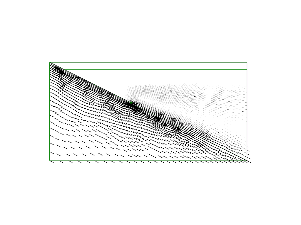
visualize it,
plotter_iso = fenics_sz.utils.plot.plot_vector_glyphs(sz_case1.vw_i, gather=True, factor=0.1, color='k', scale=fenics_sz.utils.mps_to_mmpyr(sz_case1.v0))
fenics_sz.utils.plot.plot_vector_glyphs(sz_case1.vs_i, gather=True, factor=0.1, color='k', scale=fenics_sz.utils.mps_to_mmpyr(sz_case1.v0), plotter=plotter_iso)
sz_case1.geom.pyvistaplot(plotter=plotter_iso, color='green', width=2)
cdpt = sz_case1.geom.slab_spline.findpoint('Slab::FullCouplingDepth')
fenics_sz.utils.plot.plot_points([[cdpt.x, cdpt.y, 0.0]], plotter=plotter_iso, render_points_as_spheres=True, point_size=10.0, color='green')
fenics_sz.utils.plot.plot_show(plotter_iso)
fenics_sz.utils.plot.plot_save(plotter_iso, output_folder / "sz_problem_case1_iso_stokes.png")
and get the diagnostic output to compare against the benchmark.
diag = sz_case1.get_diagnostics()

print('')
print('{:<12} {:<12} {:<12}'.format('resscale', 'T_ndof', 'Vrmsw'))
print('{:<12.4g} {:<12d} {:<12.4f}'.format(resscale, diag['T_ndof'], diag['Vrmsw']))
resscale     T_ndof       Vrmsw
5            5812         34.6379
For comparison the \(V^*_{\text{rms},w}\) values reported for case 1 using TerraFERMA in Wilson & van Keken, 2023 are:
|
\(T_{\text{ndof}} \) |
\(V_{\text{rms},w}^*\) |
|---|---|---|
2.0 |
21403 |
34.64 |
1.0 |
83935 |
34.64 |
0.5 |
332307 |
34.64 |
so even though we are at lower resolution our velocity solution appears to be reasonably good in this case.
This is just intended as an initial test and demonstration and we will perform more benchmark testing later once we have a full solution. In the next notebook we will implement the temperature equation for a steady-state problem.