Subduction Zone Model Setup#
Implementation#
As a reminder our implementation is following a similar workflow to that seen in the background examples.
we will describe the subduction zone geometry and tesselate it into non-overlapping triangles to create a mesh
we will declare function spaces for the temperature, wedge velocity and pressure, and slab velocity and pressure
using these function spaces we will declare trial and test functions
we will define Dirichlet boundary conditions at the boundaries as described in the introduction
we will describe discrete weak forms for temperature and each of the coupled velocity-pressure systems that will be used to assemble the matrices (and vectors) to be solved
we will set up matrices and solvers for the discrete systems of equations
we will solve the matrix problems
We are at step 1. Even in the simplified case, the geometry of a subduction zone is more complicated than any of the in built meshes provided to us by dolfinx. In kinematic slab models we need to describe the slab and the surrounding domain around it, including crustal layers and surface features. We are particularly interested in the dynamics near the mantle wedge corner in the sub-arc region so will employ variable resolutions, with refined cells in this area. Luckily, finite elements excel at describing these more complicated, variable resolution geometries using unstructured meshes.
Due to this complication, in this notebook we only tackle the first part of step 1, implementing a function that describes the slab surface using a spline. Since the geometry is not our primary concern here we utilize classes provided in the python/fenics_sz/geometry.py module for much of the implementation.
Preamble#
Let’s start by adding the path to the modules in the python folder to the system path (so we can find the geometry module).
import sys, os
basedir = ''
if "__file__" in globals(): basedir = os.path.dirname(__file__)
sys.path.insert(0, os.path.join(basedir, os.path.pardir, os.path.pardir, 'python'))
Let’s also load the module generated by the previous notebook to get access to the default parameters loaded there.
from fenics_sz.sz_problems.sz_params import default_params, allsz_params
Then let’s load all the remaining required modules at the beginning and set up a default output directory.
import fenics_sz.geometry as geo
from mpi4py import MPI
import matplotlib.pyplot as pl
import pathlib
output_folder = pathlib.Path(os.path.join(basedir, "output"))
output_folder.mkdir(exist_ok=True, parents=True)
Slab geometry#
In kinematic slab models the slab is typically described using a small number of points derived from seismic data which are then fitted with a spline to interpolate and extrapolate the geometry to other depths. We will use a cubic spline provided by the scipy module and wrapped for convenience in our own python/fenics_sz/geometry.py python module. We need to provide the points describing the spline, some information about the resolution we desire in the mesh at various points along the spline, and information about some points that we require to be included in the spline. The most important of these are the coupling depth (coupling_depth), at which coupling begins, and the depth at which full coupling occurs (calculated here from coupling_depth + coupling_depth_range). Both coupling_depth and coupling_depth_range were previously loaded in default_params and will later be used as the depths that determine where the slab becomes coupled to the mantle wedge. These parameters are key in determining the subduction zone thermal structure. We also include a point at slab_det_depth that we use to extract diagnostic information.
We set up the slab using the function create_slab below.
def create_slab(xs, ys, resscale, lc_depth,
                **kwargs):
    """
    Function to construct and return a spline object that is used to describe a subducting slab
    in a kinematic-slab model of a subduction zone.  Optional keyword arguments default to parameters
    in the global default_params dictionary if not specified.

    Arguments:
      * xs             - list of x points in slab spline
      * ys             - list of y points in slab spline (must be the same length as xs)
      * resscale       - resolution scale factor that multiplies all _res_fact parameters
      * lc_depth       - depth of lower crustal boundary ("Moho")

    Keyword Arguments:
     distances:
      * slab_diag1_depth - starting depth of slab diagnostic region
      * slab_diag2_depth - end depth of slab diagnostic region
      * coupling_depth   - partial coupling depth on slab
      * coupling_depth_range - depth range over which slab goes from being partially to fully coupled
      * slab_det_depth       - detector depth on slab

     resolutions factors (that get multiplied by the resscale to get the resolutions):
      * partial_coupling_depth_res_fact - partial coupling depth on slab
      * full_coupling_depth_res_fact    - full coupling depth on slab

     surface ids:
      * fault_sid            - fault
      * slab_sid             - default slab surface id
      * slab_diag_sid        - diagnostic region of slab

    Returns:
      * slab - subduction zone slab spline instance
    """

    # get input parameters
    # depths
    slab_diag1_depth       = kwargs.get('slab_diag1_depth', default_params['slab_diag1_depth'])
    slab_diag2_depth       = kwargs.get('slab_diag2_depth', default_params['slab_diag2_depth'])
    partial_coupling_depth = kwargs.get('coupling_depth', default_params['coupling_depth'])
    full_coupling_depth    = partial_coupling_depth + kwargs.get('coupling_depth_range', default_params['coupling_depth_range'])
    slab_det_depth         = kwargs.get('slab_det_depth', default_params['slab_det_depth'])

    # resolutions
    partial_coupling_depth_res = kwargs.get('partial_coupling_depth_res_fact', default_params['partial_coupling_depth_res_fact'])*resscale
    full_coupling_depth_res    = kwargs.get('full_coupling_depth_res_fact', default_params['full_coupling_depth_res_fact'])*resscale

    # surface ids
    fault_sid      = kwargs.get('fault_sid', default_params['fault_sid'])
    slab_sid       = kwargs.get('slab_sid', default_params['slab_sid'])
    slab_diag_sid  = kwargs.get('slab_diag_sid', default_params['slab_diag_sid'])

    # set up resolutions along the slab depending on depth
    # high resolution at shallow depths, lower resolution below the "diagnostic"
    # region required in the benchmark case
    # FIXME: these are currently hard-coded relative to the resolutions specified at the partial and full coupling
    # depths for simplicity but could be separate parameters
    res = [partial_coupling_depth_res if y >= -slab_diag2_depth else 3*full_coupling_depth_res for y in ys]

    # set up the surface ids for the slab depending on depth
    # above the "Moho" use fault_sid
    # in the diagnostic region use the slab_diag_sid
    # everywhere else use the default slab_sid
    sids = []
    for y in ys[1:]:
        if y >= -lc_depth:
            sid = fault_sid
        elif y >= -slab_diag1_depth:
            sid = slab_sid
        elif y >= -slab_diag2_depth:
            sid = slab_diag_sid
        else:
            sid = slab_sid
        sids.append(sid)

    # set up the slab spline object
    slab = geo.SlabSpline(xs, ys, res=res, sid=sids, name="Slab")

    assert(full_coupling_depth > partial_coupling_depth)
    # adding the coupling depths may or may not be necessary
    # depending on if they were included in the slab spline data already or not
    # the slab class should ignore them if they aren't necessary
    slab.addpoint(partial_coupling_depth, "Slab::PartialCouplingDepth",
                  res=partial_coupling_depth_res,
                  sid=slab_diag_sid)
    slab.addpoint(full_coupling_depth, "Slab::FullCouplingDepth",
                  res=full_coupling_depth_res,
                  sid=slab_diag_sid)
    # add the slab detector point
    slab.addpoint(slab_det_depth, "Slab::DetectorPoint",
                  res=full_coupling_depth_res,
                  sid=slab_diag_sid)

    # and return it
    return slab
Demonstration - Benchmark#
Describing the slab geometry only takes a few non-default parameters, which are relatively simple in the simplified benchmark geometry.
Although the resolution of our mesh is going to vary across the domain we will use a resolution scale factor resscale to scale the resolution globally, while different points in the domain retain the same default relative resolutions. So a large resscale means low resolution and a small resscale means high resolution.
Computational cost
Setting the resscale too low will result in a computationally expensive simulation, especially in the non-linear case, that may need to be run locally rather than online.
resscale = 5.0
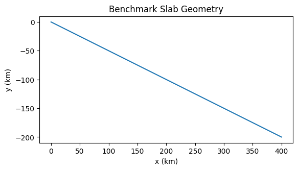
The benchmark slab geometry is rather simple, just consisting of a straight line with 2:1 horizontal distance to depth ratio, extending to 200 km depth. We can therefore just provide the spline with a series of linearly related points xs and ys.
# points in slab (just linear)
xs = [0.0, 140.0, 240.0, 400.0]
ys = [0.0, -70.0, -120.0, -200.0]
To get the surface ids on the slab correct we also have to provide the lower crustal depth lc_depth. As this is a case dependent parameter it is not provided in default_params. For the benchmark cases it is at 40 km depth.
lc_depth = 40
Providing these parameters we can create our slab geometry.
slab = create_slab(xs, ys, resscale, lc_depth)
We can double check that it looks as expected by plotting the slab, though in the benchmark case this is not very interesting!
def plot_slab(slab):
    """
    A python function to plot the given slab and return a matplotlib figure.
    """
    interpx = [curve.points[0].x for curve in slab.interpcurves]+[slab.interpcurves[-1].points[1].x]
    interpy = [curve.points[0].y for curve in slab.interpcurves]+[slab.interpcurves[-1].points[1].y]
    fig = pl.figure()
    ax = fig.gca()
    ax.plot(interpx, interpy)
    ax.set_xlabel('x (km)')
    ax.set_ylabel('y (km)')
    ax.set_aspect('equal')
    ax.set_title('Slab Geometry')
    return fig
fig = plot_slab(slab)
fig.gca().set_title('Benchmark Slab Geometry')
fig.savefig(output_folder / 'sz_slab_benchmark.png')
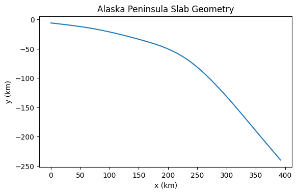
Demonstration - Alaska Peninsula#
Since the benchmark slab geometry is not very interesting we can also demonstrate the create_slab function on a more interesting case from the global suite, “01_Alaska_Peninsula”.
resscale = 5.0
szdict_ak = allsz_params['01_Alaska_Peninsula']
slab_ak = create_slab(szdict_ak['xs'], szdict_ak['ys'], resscale, szdict_ak['lc_depth'])
and plot the resulting geometry
fig = plot_slab(slab_ak)
fig.gca().set_title('Alaska Peninsula Slab Geometry')
pl.savefig(output_folder / 'sz_slab_ak.png')
While this won’t be fully tested until we compare against existing simulations, create_slab appears to be working and we can move on to describing the rest of the subduction zone geometry in the next notebook.