Subduction Zone Model Setup#
Implementation#
Our implementation will follow a similar workflow to that seen in the background examples.
we will describe the subduction zone geometry and tesselate it into non-overlapping triangles to create a mesh
we will declare function spaces for the temperature, wedge velocity and pressure, and slab velocity and pressure
using these function spaces we will declare trial and test functions
we will define Dirichlet boundary conditions at the boundaries as described in the introduction
we will describe discrete weak forms for temperature and each of the coupled velocity-pressure systems that will be used to assemble the matrices (and vectors) to be solved
we will set up matrices and solvers for the discrete systems of equations
we will solve the matrix problems
The only difference in a subduction zone problem is that each of these steps is more complicated than in the earlier examples. Here we split steps 1-7 up across several notebooks. In the first we implement a python function to describe the slab surface using a spline. The remaining details of the geometry are constructed in a function defined in the next notebook. Finally we implement a series of python classes to describe the remaining steps, 2-7, of the problem across subsequent notebooks.
Geometry#
Throughout our implementation, in the following notebooks, we will demonstrate its functionality using the simplified geometry previously laid out and repeated below in Figure 3.2.1. However our implementation will be applicable to the broader range of geometries and setups seen in the global suite.
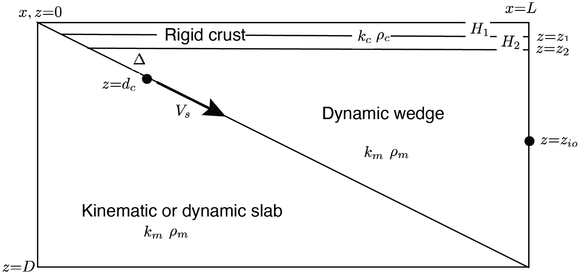 Figure 3.2.1: Geometry and coefficients for a simplified 2D subduction zone model. All coefficients and parameters are nondimensional. The decoupling point is indicated by the circle on the slab.
Parameters#
We also recall the default parameters repeated below in Table 3.2.1.
Quantity |
Symbol |
Nominal value |
Nondimensional value |
|---|---|---|---|
Reference temperature scale |
\( T_0\) |
1 K=1\(^\circ\)C |
- |
Surface temperature |
\(T^*_s\) |
273 K=0\(^\circ\)C |
\(T_s\)=0 |
Mantle temperature |
\(T^*_m\) |
1623 K=1350\(^\circ\)C |
\(T_m\)=1350 |
Surface heat flow\(^\text{c}\) |
\(q^*_s\) |
\(^\S\) W/m\(^2\) |
\(q_s\)\(^\S\) |
Reference density |
\(\rho_0\) |
3300 kg/m\(^3\) |
- |
Crustal density\(^\text{c}\) |
\(\rho^*_c\) |
2750 kg/m\(^3\) |
\(\rho_c\)=0.833333 |
Mantle density |
\(\rho^*_m\) |
3300 kg/m\(^3\) |
\(\rho_m\)=1 |
Reference thermal conductivity |
\(k_0\) |
3.1 W/(m K) |
- |
Crustal thermal conductivity\(^\text{c}\) |
\(k^*_c\) |
2.5 W/(m K) |
\(k_c\)=0.8064516 |
Mantle thermal conductivity |
\(k^*_m\) |
3.1 W/(m K) |
\(k_m\)=1 |
Volumetric heat production (upper crust)\(^\text{c}\) |
\(H^*_1\) |
1.3 \(\mu\)W/m\(^3\) |
\(H_1\)=0.419354 |
Volumetric heat production (lower crust)\(^\text{c}\) |
\(H_2^*\) |
0.27 \(\mu\)W/m\(^3\) |
\(H_2\)=0.087097 |
Age of overriding crust\(^\text{o}\) |
\(A_c^*\) |
\(^\S\) Myr |
\(A_c\)\(^\S\) |
Age of subduction\(^\text{t}\) |
\(A_s^*\) |
\(^\S\) Myr |
\(A_s\)\(^\S\) |
Age of subducting slab |
\(A^*\) |
\(^\S\) Myr |
\(A\)\(^\S\) |
Reference length scale |
\(h_0\) |
1 km |
- |
Depth of base of upper crust\(^\text{c}\) |
\(z_1^*\) |
15 km |
\(z_1\)=15 |
Depth of base of lower crust (Moho) |
\(z_2^*\) |
\(^\S\) km |
\(z_2\)\(^\S\) |
Trench depth |
\(z_\text{trench}^*\) |
\(^\S\) km |
\(z_\text{trench}\)\(^\S\) |
Position of the coast line |
\(x_\text{coast}^*\) |
\(^\S\) km |
\(x_\text{coast}\)\(^\S\) |
Wedge inflow/outflow transition depth |
\(z_\text{io}^*\) |
\(^\S\) km |
\(z_\text{io}\)\(^\S\) |
Depth of domain |
\(D^*\) |
\(^\S\) km |
\(D\)\(^\S\) |
Width of domain |
\(L^*\) |
\(^\S\) km |
\(L\)\(^\S\) |
Depth of change from decoupling to coupling |
\(d_c^*\) |
80 km |
\(d_c\)=80 |
Depth range of partial to full coupling |
\(\Delta d_c^*\) |
2.5 km |
\(\Delta d_c\)=2.5 |
Reference heat capacity |
\({c_p}_0\) |
1250 J/(kg K) |
- |
Reference thermal diffusivity |
\(\kappa_0\) |
0.7515\(\times\)10\(^{\textrm{-6}}\) m\(^2\)/s |
- |
Activation energy |
\(E\) |
540 kJ/mol |
- |
Powerlaw exponent |
\(n\) |
3.5 |
- |
Pre-exponential constant |
\(A^*_\eta\) |
28968.6 Pa s\(^{1/n}\) |
- |
Reference viscosity scale |
\(\eta_0\) |
10\(^{\textrm{21}}\) Pa s |
- |
Viscosity cap |
\(\eta^*_\text{max}\) |
10\(^{\textrm{25}}\) Pa s |
- |
Gas constant |
\(R^*\) |
8.3145 J/(mol K) |
- |
Derived velocity scale |
\({v}_0\) |
23.716014 mm/yr |
- |
Convergence velocity |
\(V_s^*\) |
\(^\S\) mm/yr |
\(V_s\)\(^\S\) |
\(^\text{c}\) |
ocean-continent subduction only |
\(^\text{o}\) |
ocean-ocean subduction only |
\(^\text{t}\) |
time-dependent simulations only |
\(^\S\) |
varies between models |
Table 3.2.1: Nomenclature and reference values
Most of these are available for us to use through a file in data/default_params.json.
import os
basedir = ''
if "__file__" in globals(): basedir = os.path.dirname(__file__)
params_filename = os.path.join(basedir, os.path.pardir, "data", "default_params.json")
Loading this file
import json
with open(params_filename, "r") as fp:
    default_params = json.load(fp)
print("{:<35} {:<10}".format('Key','Value'))
print("-"*45)
for k, v in default_params.items():
    print("{:<35} {:<10}".format(k, v))
Key                                 Value
---------------------------------------------
slab_sid                            1
slab_side_sid                       2
wedge_side_sid                      3
upper_wedge_side_sid                4
lc_side_sid                         5
uc_side_sid                         6
slab_base_sid                       7
wedge_base_sid                      8
lc_base_sid                         9
uc_base_sid                         10
coast_sid                           11
top_sid                             12
fault_sid                           13
slab_diag_sid                       14
slab_rid                            1
wedge_rid                           2
lc_rid                              3
uc_rid                              4
wedge_diag_rid                      5
slab_det_depth                      100.0
coupling_depth                      80.0
coupling_depth_range                2.5
slab_diag1_depth                    70.0
slab_diag2_depth                    120.0
partial_coupling_depth_res_fact     1.0
full_coupling_depth_res_fact        1.0
io_depth_res_fact                   4.0
coast_res_fact                      1.0
lc_side_res_fact                    2.0
lc_slab_res_fact                    1.0
slab_side_base_res_fact             8.0
uc_side_res_fact                    2.0
uc_slab_res_fact                    1.0
wedge_side_top_res_fact             4.0
wedge_side_base_res_fact            4.0
slab_diag1_res_fact                 1.0
slab_diag2_res_fact                 1.0
This contains default parameters required to define the geometry. Keys ending in _sid and _rid are surface and region IDs respectively that we use to identify boundaries and regions of the mesh (these are unlikely to need to be changed). *_res_fact are resolution factors scaled by a factor to set the resolution at various points in the mesh. Finally, those ending in _depth are depths (in km) of various important points along the slab surface or boundaries (as defined in Table 3.2.1).
We will additionally use parameters from the benchmark proposed in Wilson & van Keken, PEPS, 2023 as defined in Table 3.2.2 below.
case |
type |
\(\eta\) |
\(q_s^*\) |
\(A^*\) |
\(z_2\) |
\(z_\text{io}\) |
\(z_\text{trench}\) |
\(x_\text{coast}\) |
\(D\) |
\(L\) |
\(V_s^*\) |
|---|---|---|---|---|---|---|---|---|---|---|---|
(W/m\(^2\)) |
(Myr) |
(mm/yr) |
|||||||||
1 |
continental |
1 |
0.065 |
100 |
40 |
139 |
0 |
0 |
200 |
400 |
100 |
2 |
continental |
\(\eta_\text{disl}\) |
0.065 |
100 |
40 |
154 |
0 |
0 |
200 |
400 |
100 |
Table 3.2.2: Benchmark parameter values
Since these benchmark parameters are so few we will simply enter them as needed. For the global suite all parameters marked as varying between models in Table 3.2.1 will change between cases. An additional database of these parameters is provided in data/all_sz.json, which we also load here
allsz_filename = os.path.join(basedir, os.path.pardir, "data", "all_sz.json")
with open(allsz_filename, "r") as fp:
    allsz_params = json.load(fp)
The allsz_params dictionary contains parameters for all 56 subduction zones organized by name
print("{}".format('Name'))
print("-"*30)
for k in allsz_params.keys():
    print("{}".format(k,))
Name
------------------------------
01_Alaska_Peninsula
02_Alaska
03_British_Columbia
04_Cascadia
05_Mexico
06_GuatElSal
07_Nicaragua
08_Costa_Rica
09_Colombia_Ecuador
10_N_Peru_Gap
11_C_Peru_Gap
12_Peru
13_N_Chile
14_NC_Chile
15_C_Chile_Gap
16_C_Chile
17_SC_Chile
18_S_Chile
19_N_Antilles
20_S_Antilles
21_Scotia
22_Aegean
23_N_Sumatra
24_C_Sumatra
25_S_Sumatra
26_Sunda_Strait
27_Java
28_Bali_Lombok
29_W_Banda_Sea
30_E_Banda_Sea
31_New_Britain
32_Solomon
33_N_Vanuatu
34_S_Vanuatu
35_Tonga
36_Kermadec
37_New_Zealand
38_S_Philippines
39_N_Philippines
40_S_Marianas
41_N_Marianas
42_Bonin
43_Izu
44_Kyushu
45_Ryukyu
46_Nankai
47_C_Honshu
48_N_Honshu
49_Hokkaido
50_S_Kurile
51_N_Kurile
52_Kamchatka
53_W_Aleutians
54_C_Aleutians
55_E_Aleutians
56_Calabria
These correspond to the locations suggested by Syracuse et al., PEPI, 2010 (see Figure 3.2.2).
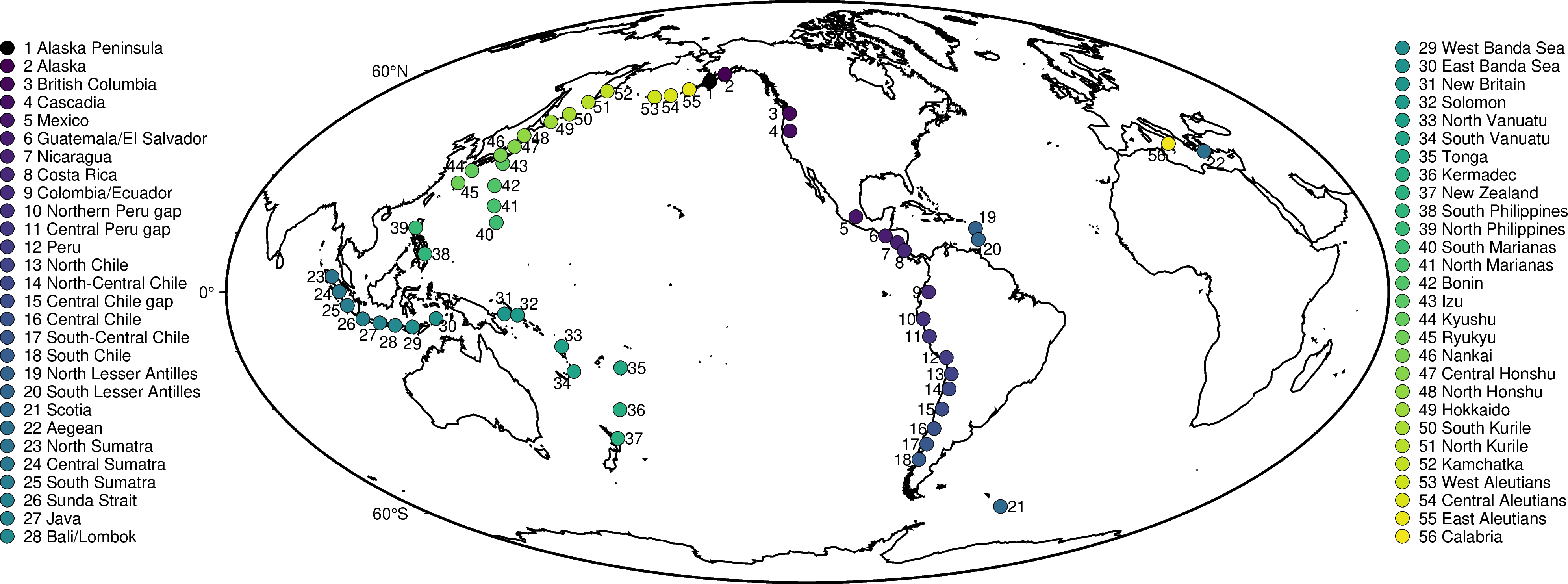
Figure 3.2.2 Locations of global suite of subduction zones, after Syracuse et al., PEPI, 2010.
Taking two examples (one continental-oceanic, “01_Alaska_Peninsula,” and one oceanic-oceanic, “19_N_Antilles”) we can examine the contents of allsz_params.
names = ['01_Alaska_Peninsula', '19_N_Antilles']
for name in names:
    print("{}:".format(name))
    print("{:<35} {:<10}".format('Key','Value'))
    print("-"*100)
    for k, v in allsz_params[name].items():
        if v is not None: print("{:<35} {}".format(k, v))
    print("="*100)
01_Alaska_Peninsula:
Key                                 Value
----------------------------------------------------------------------------------------------------
coast_distance                      260
extra_width                         20
lc_depth                            35
io_depth                            185
uc_depth                            15
dirname                             01_Alaska_Peninsula
As                                  40.0
qs                                  0.065
A                                   52.2
sztype                              continental
Vs                                  59.0
z0                                  0.8
z15                                 0.4
xs                                  [0, 68.2, 154.2, 235.0, 248.0, 251.0, 270.0, 358.0, 392.0]
ys                                  [-6, -15.0, -35.0, -70.0, -80.0, -82.5, -100.0, -200.0, -240.0]
====================================================================================================
19_N_Antilles:
Key                                 Value
----------------------------------------------------------------------------------------------------
coast_distance                      185
extra_width                         19
lc_depth                            30
io_depth                            172
dirname                             19_N_Antilles
As                                  40.0
Ac                                  90.0
A                                   85
sztype                              oceanic
Vs                                  17.6
z0                                  0.5
z15                                 0.25
xs                                  [0, 50.0, 102.2, 166.0, 176.5, 179.0, 195.0, 271.0, 301.0]
ys                                  [-6, -15.0, -30.0, -70.0, -80.0, -82.5, -100.0, -200.0, -240.0]
====================================================================================================
In the next notebook we will use some of these parameters to define the slab geometry, as the first step in describing the geometry of the whole domain.