26 Sunda Strait#
Steady state implementation#
Preamble#
We are going to run this notebook in parallel using ipyparallel. To do this we launch a parallel engine with nprocs processes. Following this, all cells we wish to run in parallel need to start with the jupyter magic %%px.
%%px
Cells without the %%px magic will run locally and will not have access to anything loaded on the parallel engine.
import ipyparallel as ipp
nprocs = 2
rc = ipp.Cluster(engine_launcher_class="mpi", n=nprocs).start_and_connect_sync()
Starting 2 engines with <class 'ipyparallel.cluster.launcher.MPIEngineSetLauncher'>
Set some path information.
%%px
import sys, os, shutil
basedir = ''
if "__file__" in globals(): basedir = os.path.dirname(__file__)
sys.path.insert(0, os.path.join(basedir, os.path.pardir, os.path.pardir, os.path.pardir, 'python'))
Loading everything we need from sz_problem and also set our default plotting and output preferences.
%%px
import fenics_sz.utils
from fenics_sz.sz_problems.sz_params import allsz_params
from fenics_sz.sz_problems.sz_slab import create_slab, plot_slab
from fenics_sz.sz_problems.sz_geometry import create_sz_geometry
from fenics_sz.sz_problems.sz_steady_dislcreep import SteadyDislSubductionProblem
import numpy as np
import dolfinx as df
import pyvista as pv
import pathlib
output_folder = pathlib.Path(os.path.join(basedir, "output"))
output_folder.mkdir(exist_ok=True, parents=True)
import hashlib
import zipfile
import requests
from mpi4py import MPI
comm = MPI.COMM_WORLD
my_rank = comm.rank
Parameters#
We first select the name and resolution scale, resscale of the model.
Resolution
By default the resolution is low to allow for a quick runtime and smaller website size. If sufficient computational resources are available set a lower resscale to get higher resolutions and results with sufficient accuracy.
%%px
name = "26_Sunda_Strait"
resscale = 3.0
Then load the remaining parameters from the global suite.
%%px
szdict = allsz_params[name]
if my_rank == 0:
    print("{}:".format(name))
    print("{:<20} {:<10}".format('Key','Value'))
    print("-"*85)
    for k, v in allsz_params[name].items():
        if v is not None and k not in ['z0', 'z15']: print("{:<20} {}".format(k, v))
[stdout:0] 26_Sunda_Strait:
Key                  Value
-------------------------------------------------------------------------------------
coast_distance       250
extra_width          17
lc_depth             33.5
io_depth             180
uc_depth             15
dirname              26_Sunda_Strait
As                   40.0
qs                   0.065
A                    85
sztype               continental
Vs                   61.0
xs                   [0, 73.7, 170.0, 240.0, 251.8, 254.5, 272.0, 352.0, 383.0]
ys                   [-6, -15.0, -33.5, -70.0, -80.0, -82.5, -100.0, -200.0, -240.0]
Any of these can be modified in the dictionary.
Several additional parameters can be modified, for details see the documentation for the SteadyDislSubductionProblem class.
%%px
if my_rank == 0: help(SteadyDislSubductionProblem.__init__)
[stdout:0] Help on function __init__ in module fenics_sz.sz_problems.sz_base:

__init__(self, geom, **kwargs)
    Initialize a BaseSubductionProblem.

    Arguments:
      * geom  - an instance of a subduction zone geometry

    Keyword Arguments:
     required:
      * A      - age of subducting slab (in Myr) [required]
      * Vs     - incoming slab speed (in mm/yr) [required]
      * sztype - type of subduction zone (either 'continental' or 'oceanic') [required]
      * Ac     - age of the overriding plate (in Myr) [required if sztype is 'oceanic']
      * As     - age of subduction (in Myr) [required if sztype is 'oceanic']
      * qs     - surface heat flux (in W/m^2) [required if sztype is 'continental']

     optional:
      * Ts   - surface temperature (deg C, corresponds to non-dim)
      * Tm   - mantle temperature (deg C, corresponds to non-dim)
      * kc   - crustal thermal conductivity (non-dim) [only has an effect if sztype is 'continental']
      * km   - mantle thermal conductivity (non-dim)
      * rhoc - crustal density (non-dim) [only has an effect if sztype is 'continental']
      * rhom - mantle density (non-dim)
      * cp   - isobaric heat capacity (non-dim)
      * H1   - upper crustal volumetric heat production (non-dim) [only has an effect if sztype is 'continental']
      * H2   - lower crustal volumetric heat production (non-dim) [only has an effect if sztype is 'continental']

     optional (dislocation creep rheology):
      * etamax - maximum viscosity (Pas) [only relevant for dislocation creep rheologies]
      * nsigma - stress viscosity power law exponents (non-dim) [only relevant for dislocation creep rheologies]
      * Aeta   - pre-exponential viscosity constant (Pa s^(1/n)) [only relevant for dislocation creep rheologies]
      * E      - viscosity activation energy (J/mol) [only relevant for dislocation creep rheologies]
Setup#
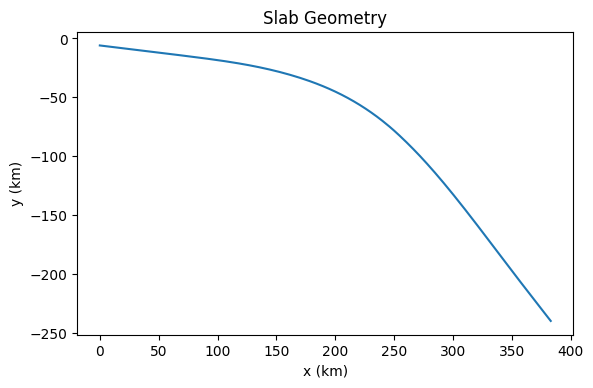
Setup a slab.
%%px
slab = create_slab(szdict['xs'], szdict['ys'], resscale, szdict['lc_depth'])
if my_rank == 0: _ = plot_slab(slab)
[output:0]
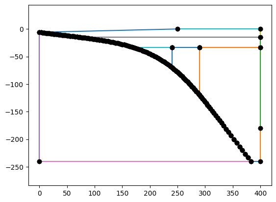
Create the subduction zome geometry around the slab.
%%px
geom = create_sz_geometry(slab, resscale, szdict['sztype'], szdict['io_depth'], szdict['extra_width'],
                             szdict['coast_distance'], szdict['lc_depth'], szdict['uc_depth'])
if my_rank == 0: _ = geom.plot()
[output:0]
Finally, declare the SubductionZone problem class using the dictionary of parameters.
%%px
sz = SteadyDislSubductionProblem(geom, **szdict)
Solve#
Solve using a dislocation creep rheology and assuming a steady state.
%%px
sz.solve()
[stdout:0] Iteration   Residual     Relative Residual
------------------------------------------
0           9540.9       1
1           3778.42      0.396024
2           209.383      0.0219459
3           93.0474      0.00975248
4           37.8292      0.00396495
5           15.4431      0.00161862
6           8.25462      0.000865182
7           5.29354      0.000554826
8           3.65009      0.000382573
9           2.60229      0.000272751
10          1.89893      0.000199031
11          1.41031      0.000147817
12          1.05998      0.000111098
13          0.803081     8.41725e-05
14          0.611794     6.41233e-05
15          0.467974     4.90493e-05
16          0.359133     3.76414e-05
17          0.276337     2.89635e-05
18          0.21314      2.23396e-05
19          0.164761     1.72689e-05
20          0.127635     1.33777e-05
21          0.0990765    1.03844e-05
22          0.0770619    8.07701e-06
23          0.0600578    6.29477e-06
24          0.0468986    4.91553e-06
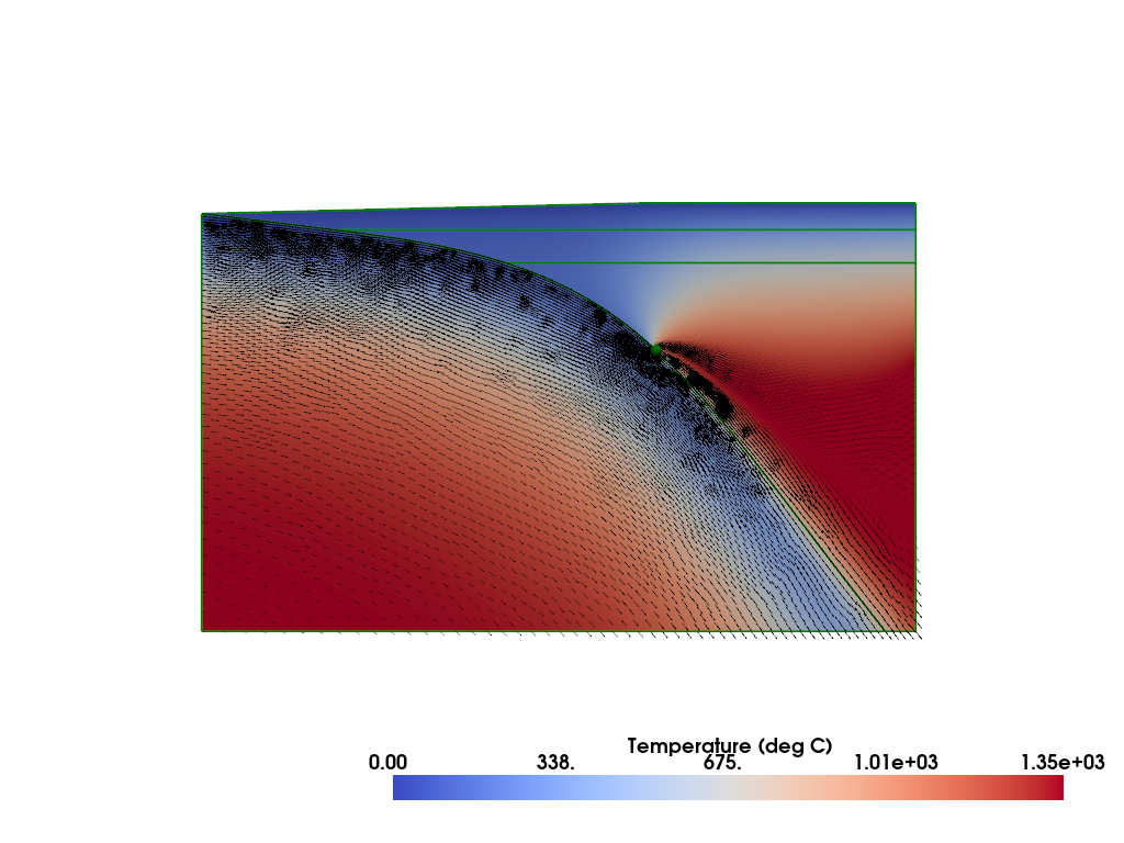
Plot#
Plot the solution.
%%px
plotter = pv.Plotter()
fenics_sz.utils.plot.plot_scalar(sz.T_i, plotter=plotter, scale=sz.T0, gather=True, cmap='coolwarm', scalar_bar_args={'title': 'Temperature (deg C)', 'bold':True})
fenics_sz.utils.plot.plot_vector_glyphs(sz.vw_i, plotter=plotter, gather=True, factor=0.1, color='k', scale=fenics_sz.utils.mps_to_mmpyr(sz.v0))
fenics_sz.utils.plot.plot_vector_glyphs(sz.vs_i, plotter=plotter, gather=True, factor=0.1, color='k', scale=fenics_sz.utils.mps_to_mmpyr(sz.v0))
geom.pyvistaplot(plotter=plotter, color='green', width=2)
cdpt = slab.findpoint('Slab::FullCouplingDepth')
fenics_sz.utils.plot.plot_points([[cdpt.x, cdpt.y, 0.0]], plotter=plotter, render_points_as_spheres=True, point_size=10.0, color='green')
if my_rank == 0:
    fenics_sz.utils.plot.plot_show(plotter)
    fenics_sz.utils.plot.plot_save(plotter, output_folder / "{}_ss_solution_resscale_{:.2f}.png".format(name, resscale))
[stderr:1] 2026-05-08 22:35:27.039 ( 15.324s) [ 7FE0A09EC140]vtkXOpenGLRenderWindow.:1416 WARN| bad X server connection. DISPLAY=:99
[stderr:0] 2026-05-08 22:35:27.037 ( 15.322s) [ 7F2AEF52F140]vtkXOpenGLRenderWindow.:1416 WARN| bad X server connection. DISPLAY=:99
[output:0]
Save it to disk so that it can be examined with other visualization software (e.g. Paraview).
%%px
filename = output_folder / "{}_ss_solution_resscale_{:.2f}.bp".format(name, resscale)
with df.io.VTXWriter(sz.mesh.comm, filename, [sz.T_i, sz.vs_i, sz.vw_i]) as vtx:
    vtx.write(0.0)
# zip the .bp folder so that it can be downloaded from jupyter lab
if my_rank == 0: shutil.make_archive(str(filename), 'zip', root_dir=str(filename.parent), base_dir=str(filename.name))
Comparison#
Compare to the published result from Wilson & van Keken, PEPS, 2023 (II) and van Keken & Wilson, PEPS, 2023 (III). The original models used in these papers are also available as open-source repositories on github and zenodo.
First download the minimal necessary data from zenodo and check it is the right version.
%%px
zipfilename = pathlib.Path(os.path.join(basedir, os.path.pardir, os.path.pardir, os.path.pardir, "data", "vankeken_wilson_peps_2023_TF_lowres_minimal.zip"))
# only one process should download the data
if my_rank == 0:
    if not zipfilename.is_file():
        zipfileurl = 'https://zenodo.org/records/13234021/files/vankeken_wilson_peps_2023_TF_lowres_minimal.zip'
        r = requests.get(zipfileurl, allow_redirects=True)
        open(zipfilename, 'wb').write(r.content)
# wait until rank 0 has downloaded the data
comm.barrier()
assert hashlib.md5(open(zipfilename, 'rb').read()).hexdigest() == 'a8eca6220f9bee091e41a680d502fe0d'
%%px
tffilename = os.path.join('vankeken_wilson_peps_2023_TF_lowres_minimal', 'sz_suite_ss', szdict['dirname']+'_minres_2.00.vtu')
tffilepath = os.path.join(basedir, os.path.pardir, os.path.pardir, os.path.pardir, 'data')
# one process should extract the file
if my_rank == 0:
    with zipfile.ZipFile(zipfilename, 'r') as z:
        z.extract(tffilename, path=tffilepath)
# other processes should wait
comm.barrier()
%%px
fxgrid = fenics_sz.utils.plot.grids_scalar(sz.T_i)[0]

tfgrid = pv.get_reader(os.path.join(tffilepath, tffilename)).read()

diffgrid = fenics_sz.utils.plot.pv_diff(fxgrid, tfgrid, field_name_map={'T':'Temperature::PotentialTemperature'}, pass_point_data=True)
%%px
# first gather the data onto rank 0
diffgrid_g = fenics_sz.utils.plot.pyvista_grids(diffgrid.cells, diffgrid.celltypes, diffgrid.points, comm, gather=True)
T_g = comm.gather(diffgrid.point_data['T'], root=0)
for r, grid in enumerate(diffgrid_g):
    grid.point_data['T'] = T_g[r]
    grid.set_active_scalars('T')
    grid.clean(tolerance=1.e-2)
diffgrid_g

# then plot it
plotter_diff = pv.Plotter()
clim = None
for grid in diffgrid_g:
    plotter_diff.add_mesh(grid, cmap='coolwarm', clim=clim, scalar_bar_args={'title': 'Temperature Difference (deg C)', 'bold':True})
geom.pyvistaplot(plotter=plotter_diff, color='green', width=2)
cdpt = slab.findpoint('Slab::FullCouplingDepth')
#fenics_sz.utils.plot.plot_points([[cdpt.x, cdpt.y, 0.0]], plotter=plotter_diff, render_points_as_spheres=True, point_size=10.0, color='green')
plotter_diff.enable_parallel_projection()
plotter_diff.view_xy()
if my_rank == 0: plotter_diff.show()
[output:0]
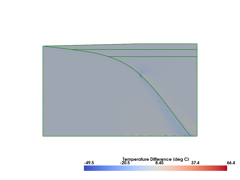
%%px
integrated_data = diffgrid.integrate_data()
totalarea = comm.allreduce(integrated_data['Area'][0], op=MPI.SUM)
error = comm.allreduce(integrated_data['T'][0], op=MPI.SUM)/totalarea
if my_rank == 0: print("Average error = {}".format(error,))
assert np.abs(error) < 5
[stdout:0] Average error = 0.384623844733862
Shutdown#
Shutdown the ipyparallel cluster engine. Running the cell below will prevent earlier cells (with %%px as the first line) from being re-run.
rc.shutdown()