Blankenbach Thermal Convection Example#
Description#
As a reminder we are seeking the approximate velocity, pressure and temperature solutions of the coupled Stokes
and heat equations
in a bottom-heated unit square domain, \(\Omega\), with boundaries, \(\partial\Omega\).
For the Stokes problem we assume free-slip boundaries
and constrain the pressure to remove its null space, e.g. by applying a reference point
For the heat equation the side boundaries are insulating, the base hot and the top cold
We seek solutions at a variety of Rayleigh numbers, Ra, and consider both isoviscous, \(\eta = 1\), cases and a case with a temperature-dependent viscosity, \(\eta(T) = \exp(-bT)\) with \(b=\ln(10^3)\).
Implementation#
This benchmark was proposed by Blankenbach et al. (1989) and has been used to test numerous models since then. One such example was presented by Wilson & van Keken, 2023 using TerraFERMA, a GUI-based model building framework that uses FEniCS v2019.1.0. Here we reproduce these results using the latest version of FEniCS, FEniCSx.
Preamble#
We start by loading all the modules we will require.
from mpi4py import MPI
import gmsh
import dolfinx as df
import dolfinx.fem.petsc
from petsc4py import PETSc
import numpy as np
import ufl
import matplotlib.pyplot as pl
import basix
import sys, os
basedir = ''
if "__file__" in globals(): basedir = os.path.dirname(__file__)
sys.path.insert(0, os.path.join(basedir, os.path.pardir, os.path.pardir, 'python'))
import fenics_sz.utils.plot
import pathlib
output_folder = pathlib.Path(os.path.join(basedir, "output"))
output_folder.mkdir(exist_ok=True, parents=True)
Solution#
We build a workflow that contains a complete description of the coupled Stokes-temperature convecting system. This follows much the same order as described in previous examples, with some modifications to solve the now nonlinearly coupled problem
in
transfinite_unit_square_meshwe use Gmsh to describe a unit square domain \(\Omega = [0,1]\times[0,1]\), tesselating it into \(2 \times\)ne\(\times\)netriangular cells, and allowing refinement near the top and bottom using the parameterbeta
def transfinite_unit_square_mesh(nx, ny, beta=1):
    """
    A python function to create a mesh of a square domain with refinement
    near the top and bottom boundaries, depending on the value of coeff.
    Parameters:
    * nx    - number of cells in the horizontal x direction
    * ny    - number of cells in the vertical y direction
    * beta  - beta mesh refinement coefficient, < 1 refines the mesh at
              the top and bottom boundaries (optional, defaults to  1, no refinement]
    Returns:
    * mesh  - the resulting mesh
    """
    # Describe the domain (a unit square)
    # and also the tessellation of that domain into ne
    # equally spaced squared in each dimension, which are
    # subduvided into two triangular elements each
    with df.common.Timer("Mesh"):
        if not gmsh.is_initialized(): gmsh.initialize()

        gmsh.model.add("square")
        # make gmsh quieter
        gmsh.option.setNumber('General.Verbosity', 3)

        lc = 1e-2  # ignored later by using transfinite curves
        # define the corners of the domain
        gmsh.model.geo.addPoint(0, 0, 0, lc, 1)
        gmsh.model.geo.addPoint(1, 0, 0, lc, 2)
        gmsh.model.geo.addPoint(1, 1, 0, lc, 3)
        gmsh.model.geo.addPoint(0, 1, 0, lc, 4)
        # define the sides of the domain
        gmsh.model.geo.addLine(1, 4, 1)
        gmsh.model.geo.addLine(2, 3, 2)
        gmsh.model.geo.addLine(1, 2, 3)
        gmsh.model.geo.addLine(4, 3, 4)
        # define the domain
        gmsh.model.geo.addCurveLoop([3, 2, -4, -1], 1)
        gmsh.model.geo.addPlaneSurface([1], 1)

        # set the boundaries as transfinite curves to allow refinement
        # and to set the resolution
        gmsh.model.geo.mesh.setTransfiniteCurve(1, ny+1, "Bump", beta)
        gmsh.model.geo.mesh.setTransfiniteCurve(2, ny+1, "Bump", beta)
        gmsh.model.geo.mesh.setTransfiniteCurve(3, nx+1)
        gmsh.model.geo.mesh.setTransfiniteCurve(4, nx+1)
        # make the mesh regular across the domain
        gmsh.model.geo.mesh.setTransfiniteSurface(1, "Left")

        gmsh.model.geo.synchronize()

        # specify some IDs (not used currently)
        gmsh.model.addPhysicalGroup(1, [1], 1)
        gmsh.model.addPhysicalGroup(1, [2], 2)
        gmsh.model.addPhysicalGroup(1, [3], 3)
        gmsh.model.addPhysicalGroup(1, [4], 4)
        gmsh.model.addPhysicalGroup(2, [1], 1)

        # generate the mesh on the first process
        if MPI.COMM_WORLD.rank == 0:
            gmsh.model.mesh.generate(2)

        # distribute and build the global mesh
        mesh = df.io.gmshio.model_to_mesh(gmsh.model, MPI.COMM_WORLD, 0, gdim=2)[0]

    return mesh
create function spaces
in
stokes_functionspaceswe declare finite elements for the velocity and pressure using Lagrange polynomials of degreepp+1andpprespectively and use these to declare function spaces,V_vandV_p, for velocity and pressurein
temperature_functionspacewe declare a finite element for the temperature using Lagrange polynomials of degreepTand use this to delcareV_T, a function space for temperature
def stokes_functionspaces(mesh, pp=1):
    """
    A python function to set up velocity and pressure function spaces.
    Parameters:
    * mesh - the mesh to set up the functions on
    * pp   - polynomial order of the pressure solution (optional, defaults to 1)
    Returns:
    * V_v  - velocity function space of polynomial order p+1
    * V_p  - pressure function space of polynomial order p
    """
    with df.common.Timer("Function spaces Stokes"):
        # Define velocity and pressure elements
        v_e = basix.ufl.element("Lagrange", mesh.basix_cell(), pp+1, shape=(mesh.geometry.dim,))
        p_e = basix.ufl.element("Lagrange", mesh.basix_cell(), pp)

        # Define the velocity and pressure function spaces
        V_v = df.fem.functionspace(mesh, v_e)
        V_p = df.fem.functionspace(mesh, p_e)

    return V_v, V_p

def temperature_functionspace(mesh, pT=1):
    """
    A python function to set up the temperature function space.
    Parameters:
    * mesh - the mesh to set up the functions on
    * pT   - polynomial order of T (optional, defaults to 1)
    Returns:
    * V_T  - temperature function space of polynomial order pT
    """
    with df.common.Timer("Function spaces Temperature"):
        # Define velocity, pressure and temperature elements
        T_e = basix.ufl.element("Lagrange", mesh.basix_cell(), pT)

        # Define the temperature function space
        V_T  = df.fem.functionspace(mesh, T_e)

    return V_T
set up boundary conditions
in
velocity_bcswe define a list of Dirichlet boundary conditions on velocityin
pressure_bcswe define a constraint on the pressure in the lower left corner of the domainin
temperature_bcswe define a list of Dirichlet boundary conditions on temperature
def velocity_bcs(V_v):
    """
    A python function to set up the velocity boundary conditions.
    Parameters:
    * V_v - velocity function space
    Returns:
    * bcs - a list of boundary conditions
    """
    with df.common.Timer("Dirichlet BCs Stokes"):
        # Define velocity sub function spaces
        V_vx, _ = V_v.sub(0).collapse()
        V_vy, _ = V_v.sub(1).collapse()

        # Declare a list of boundary conditions for the Stokes problem
        bcs = []

        # Define the location of the left and right boundary and find the x-velocity DOFs
        def boundary_leftandright(x):
            return np.logical_or(np.isclose(x[0], 0), np.isclose(x[0], 1))
        dofs_vx_leftright = df.fem.locate_dofs_geometrical((V_v.sub(0), V_vx), boundary_leftandright)
        # Specify the velocity value and define a Dirichlet boundary condition
        zero_vx = df.fem.Function(V_vx)
        zero_vx.x.array[:] = 0.0
        bcs.append(df.fem.dirichletbc(zero_vx, dofs_vx_leftright, V_v.sub(0)))

        # Define the location of the top and bottom boundary and find the y-velocity DOFs
        def boundary_topandbase(x):
            return np.logical_or(np.isclose(x[1], 0), np.isclose(x[1], 1))
        dofs_vy_topbase = df.fem.locate_dofs_geometrical((V_v.sub(1), V_vy), boundary_topandbase)
        zero_vy = df.fem.Function(V_vy)
        zero_vy.x.array[:] = 0.0
        bcs.append(df.fem.dirichletbc(zero_vy, dofs_vy_topbase, V_v.sub(1)))

    return bcs

def pressure_bcs(V_p):
    """
    A python function to set up the pressure boundary conditions.
    Parameters:
    * V_p - pressure function space
    Returns:
    * bcs - a list of boundary conditions
    """
    with df.common.Timer("Dirichlet BCs Stokes"):
        # Declare a list of boundary conditions
        bcs = []

        # Grab the mesh
        mesh = V_p.mesh

        # Define the location of the lower left corner of the domain and find the pressure DOF there
        def corner_lowerleft(x):
            return np.logical_and(np.isclose(x[0], 0), np.isclose(x[1], 0))
        dofs_p_lowerleft = df.fem.locate_dofs_geometrical(V_p, corner_lowerleft)
        # Specify the arbitrary pressure value and define a Dirichlet boundary condition
        zero_p = df.fem.Constant(mesh, df.default_scalar_type(0.0))
        bcs.append(df.fem.dirichletbc(zero_p, dofs_p_lowerleft, V_p))

    return bcs

def temperature_bcs(V_T):
    """
    A python function to set up the temperature boundary conditions.
    Parameters:
    * V_T - temperature function space
    Returns:
    * bcs - a list of boundary conditions
    """
    with df.common.Timer("Dirichlet BCs Temperature"):
        # Declare a list of boundary conditions for the temperature problem
        bcs = []

        # Grab the mesh
        mesh = V_T.mesh

        # Define the location of the top boundary and find the temperature DOFs
        def boundary_top(x):
            return np.isclose(x[1], 1)
        dofs_T_top = df.fem.locate_dofs_geometrical(V_T, boundary_top)
        zero_T = df.fem.Constant(mesh, df.default_scalar_type(0.0))
        bcs.append(df.fem.dirichletbc(zero_T, dofs_T_top, V_T))

        # Define the location of the base boundary and find the temperature DOFs
        def boundary_base(x):
            return np.isclose(x[1], 0)
        dofs_T_base = df.fem.locate_dofs_geometrical(V_T, boundary_base)
        one_T = df.fem.Constant(mesh, df.default_scalar_type(1.0))
        bcs.append(df.fem.dirichletbc(one_T, dofs_T_base, V_T))

    return bcs
declare discrete weak forms
stokes_weakformsuses the velocity and pressure function spaces to declare trial,v_aandp_a, and test,v_tandp_t, functions for the velocity and pressure respectively and uses them to describe the discrete weak forms,Sandf, that will be used to assemble the matrix \(\mathbf{S}_m\) and vector \(\mathbf{f}_m\)we also implement a dummy weak form for the pressure block in
dummy_pressure_weakformthat allows us to apply a pressure boundary conditionthe weak form for a pressure mass matrix scaled by the inverse of the viscosity in
pressure_preconditioner_weakformis used to precondition the zero block of the Stokes matrix when using an iterative solvertemperature_weakformscreates weak forms for the steady-state advection-diffusion temperature equation
def stokes_weakforms(v, p, T, Ra, b=None):
    """
    A python function to return the weak forms for the Stokes problem.
    By default this assumes an isoviscous rheology but supplying b allows
    a temperature dependent viscosity to be used.
    Parameters:
    * v   - velocity function
    * p   - pressure function
    * T   - the temperature finite element function
    * Ra  - Rayleigh number
    * b   - temperature dependence of viscosity (optional, defaults to isoviscous)
    Returns:
    * S   - a bilinear form
    * f   - a linear form
    * r   - a linear form for the residual
    """
    with df.common.Timer("Forms Stokes"):
        # Grab the velocity-pressure function space and the mesh
        V_v = v.function_space
        V_p = p.function_space
        mesh = V_p.mesh

        # Define extra constants
        Ra_c = df.fem.Constant(mesh, df.default_scalar_type(Ra))
        gravity = df.fem.Constant(mesh, df.default_scalar_type((0.0,-1.0)))
        eta = 1
        if b is not None:
            b_c  = df.fem.Constant(mesh, df.default_scalar_type(b))
            eta = ufl.exp(-b_c*T)

        # Define the trial functions for velocity and pressure
        v_a, p_a = ufl.TrialFunction(V_v), ufl.TrialFunction(V_p)
        # Define the test functions for velocity and pressure
        v_t, p_t = ufl.TestFunction(V_v),  ufl.TestFunction(V_p)

        # Define the integrals to be assembled into the stiffness matrix for the Stokes system
        K = ufl.inner(ufl.sym(ufl.grad(v_t)), 2*eta*ufl.sym(ufl.grad(v_a)))*ufl.dx
        G = -ufl.div(v_t)*p_a*ufl.dx
        D = -p_t*ufl.div(v_a)*ufl.dx
        S = [[K, G], [D, None]]

        # Define the integral to the assembled into the forcing vector for the Stokes system
        zero_p = df.fem.Constant(mesh, df.default_scalar_type(0.0))
        f = [-ufl.inner(v_t, gravity)*Ra_c*T*ufl.dx, zero_p*p_t*ufl.dx]

        # define the residual
        r = [ufl.action(S[0][0], v) + ufl.action(S[0][1], p) - f[0], ufl.action(S[1][0], v) - f[1]]

    return df.fem.form(S), df.fem.form(f), df.fem.form(r)

def dummy_pressure_weakform(p):
    """
    A python function to return a dummy (zero) weak form for the pressure block of
    the Stokes problem.
    Parameters:
    * p   - pressure function
    Returns:
    * M   - a bilinear form
    """
    with df.common.Timer("Forms Stokes"):
        # Grab the function space and mesh
        V_p = p.function_space
        mesh = V_p.mesh

        # Define the trial function for the pressure
        p_a = ufl.TrialFunction(V_p)
        # Define the test function for the pressure
        p_t = ufl.TestFunction(V_p)

        # Define the dummy integrals to be assembled into a zero pressure mass matrix
        zero_p = df.fem.Constant(mesh, df.default_scalar_type(0.0))
        M = p_t*p_a*zero_p*ufl.dx

    return df.fem.form(M)

def pressure_preconditioner_weakform(p, T, b=None):
    """
    A python function to return a weak form for the pressure preconditioner of
    the Stokes problem.
    Parameters:
    * p   - pressure function
    * T   - the temperature finite element function
    * b   - temperature dependence of viscosity (optional, defaults to isoviscous)
    Returns:
    * M   - a bilinear form
    """
    with df.common.Timer("Forms Stokes"):
        # Grab the function space and mesh
        V_p = p.function_space
        mesh = V_p.mesh

        # Define extra constants
        inveta = 1
        if b is not None:
            b_c  = df.fem.Constant(mesh, df.default_scalar_type(b))
            inveta = ufl.exp(b_c*T)

        # Define the trial function for the pressure
        p_a = ufl.TrialFunction(V_p)
        # Define the test function for the pressure
        p_t = ufl.TestFunction(V_p)

        # Define the integrals to be assembled into a pressure mass matrix
        M = inveta*p_t*p_a*ufl.dx

    return df.fem.form(M)

def temperature_weakforms(T, v):
    """
    A python function to return the weak forms for the temperature problem.
    Parameters:
    * T   - the temperature function space
    * v   - the velocity function
    Returns:
    * S   - a bilinear form
    * f   - a linear form
    * r   - a linear form for the residual
    """
    with df.common.Timer("Forms Temperature"):
        # Grab the function space and mesh
        V_T = T.function_space
        mesh = V_T.mesh

        # Define the temperature test function
        T_t = ufl.TestFunction(V_T)

        # Define the temperature trial function
        T_a = ufl.TrialFunction(V_T)

        # Define the integrals to be assembled into the stiffness matrix for the temperature system
        S = (T_t*ufl.inner(v, ufl.grad(T_a)) + ufl.inner(ufl.grad(T_t), ufl.grad(T_a)))*ufl.dx

        # Define the integral to the assembled into the forcing vector for the temperature system
        # which in this case is just zero
        f = df.fem.Constant(mesh, df.default_scalar_type(0.0))*T_t*ufl.dx

        # Define the residual
        r = ufl.action(S, T) - f

    return df.fem.form(S), df.fem.form(f), df.fem.form(r)
We approach assembly and solving slightly differently than before because we will be calling the solvers multiple times. Here we combine elements of the assembly and solution steps to do the initial set up - declaring and configuring the matrices, assembling those blocks that won’t change at each iteration and finally declaring and returning a solver.
setup_stokes_solver_nestsets up a PETSc MATNEST matrix and (if necessary) preconditioner matrix and assembles any blocks that do not change in the Picard iteration before attaching them to a PETSc KSP linear solver object and returning it along with vectors for the RHS and residualsetup_temperature_solverdoes the same for the temperature equations (but performs no pre-assembly because it will always need to be assembled in the nonlinear loop owing to its dependence on velocity)
def setup_stokes_solver_nest(S, f, r, bcs, M=None, isoviscous=False,
                             attach_nullspace=False, attach_nearnullspace=True):
    """
    A python function to create a nested matrix and a vector for the given Stokes forms.
    Parameters:
    * S   - Stokes bilinear form
    * f   - Stokes RHS linear form
    * r   - Stokes residual form
    * bcs - list of Stokes boundary conditions
    * M   - viscosity weighted pressure mass matrix bilinear form (optional, defaults to None)
    * isoviscous - if isoviscous assemble the velocity/pressure mass block at setup (optional, defaults to False)
    * attach_nullspace - attach the pressure nullspace to the matrix (optional, defaults to False)
    * attach_nearnullspace - attach the possible (near) velocity nullspaces to the preconditioning matrix
                             (optional, defaults to True)
    Returns:
    * solver - a PETSc KSP solver object
    * fm     - rhs vector
    * rm     - residual vector
    """

    # retrieve the petsc options
    opts = PETSc.Options()
    pc_type = opts.getString('stokes_pc_type')

    with df.common.Timer("Assemble Stokes"):
        # create the matrix
        Sm = df.fem.petsc.create_matrix_nest(S)
        # set a flag to indicate that the velocity block is
        # symmetric positive definite (SPD)
        Sm00 = Sm.getNestSubMatrix(0, 0)
        Sm00.setOption(PETSc.Mat.Option.SPD, True)

        def assemble_block(i, j):
            if S[i][j] is not None:
                Smij = Sm.getNestSubMatrix(i, j)
                Smij.zeroEntries()
                Smij = df.fem.petsc.assemble_matrix(Smij, S[i][j], bcs=bcs)

        # these blocks don't change so only assemble them here
        assemble_block(0, 1)
        assemble_block(1, 0)
        assemble_block(1, 1)
        # only assemble velocity block if we're isoviscous and we
        # won't be assembling it in the Picard iterations
        if isoviscous:
            assemble_block(0, 0)
            Sm.assemble()

        # create the RHS vector
        fm = df.fem.petsc.create_vector_nest(f)

        # create the residual vector
        rm = df.fem.petsc.create_vector_nest(r)

        if attach_nullspace:
            V_p_cpp = df.fem.extract_function_spaces(f)[1]
            # set up a null space vector indicating the null space
            # in the pressure DOFs
            null_vec = df.fem.petsc.create_vector_nest(f)
            null_vecs = null_vec.getNestSubVecs()
            null_vecs[0].set(0.0)
            null_vecs[1].set(1.0)
            null_vec.normalize()
            ns = PETSc.NullSpace().create(vectors=[null_vec], comm=V_p_cpp.mesh.comm)
            Sm.setNullSpace(ns)

        # assemble the pre-conditioner (if M was supplied)
        Pm = None
        if M is not None:
            Mm = df.fem.petsc.create_matrix(M)

            Pm = PETSc.Mat().createNest([[Sm.getNestSubMatrix(0, 0), None], [None, Mm]])

            # set the SPD flag on the diagonal blocks of the preconditioner
            Pm00, Pm11 = Pm.getNestSubMatrix(0, 0), Pm.getNestSubMatrix(1, 1)
            Pm00.setOption(PETSc.Mat.Option.SPD, True)
            Pm11.setOption(PETSc.Mat.Option.SPD, True)

            # only assemble the mass matrix block if we're isoviscous
            # and we won't be assembling it in the Picard iterations
            if isoviscous:
                Mm = df.fem.petsc.assemble_matrix(Mm, M, bcs=bcs)
                Mm.assemble()
                Pm.assemble()

            if attach_nearnullspace:
                V_v_cpp = df.fem.extract_function_spaces(f)[0]

                bs = V_v_cpp.dofmap.index_map_bs
                length0 = V_v_cpp.dofmap.index_map.size_local
                ns_basis = [df.la.vector(V_v_cpp.dofmap.index_map, bs=bs, dtype=PETSc.ScalarType) for i in range(3)]
                ns_arrays = [ns_b.array for ns_b in ns_basis]

                dofs = [V_v_cpp.sub([i]).dofmap.map().flatten() for i in range(bs)]

                # Set the three translational rigid body modes
                for i in range(2):
                    ns_arrays[i][dofs[i]] = 1.0

                x = V_v_cpp.tabulate_dof_coordinates()
                dofs_block = V_v_cpp.dofmap.map().flatten()
                x0, x1 = x[dofs_block, 0], x[dofs_block, 1]
                ns_arrays[2][dofs[0]] = -x1
                ns_arrays[2][dofs[1]] = x0

                df.la.orthonormalize(ns_basis)

                ns_basis_petsc = [PETSc.Vec().createWithArray(ns_b[: bs * length0], bsize=bs, comm=V_v_cpp.mesh.comm) for ns_b in ns_arrays]
                nns = PETSc.NullSpace().create(vectors=ns_basis_petsc, comm=V_v_cpp.mesh.comm)
                Pm00.setNearNullSpace(nns)

    with df.common.Timer("Solve Stokes"):
        solver = PETSc.KSP().create(MPI.COMM_WORLD)
        solver.setOperators(Sm, Pm)
        solver.setOptionsPrefix("stokes_")
        solver.setFromOptions()

        # a fieldsplit preconditioner allows us to precondition
        # each block of the matrix independently but we first
        # have to set the index sets (ISs) of the DOFs on which
        # each block is defined
        if pc_type == "fieldsplit":
            iss = Pm.getNestISs()
            solver.getPC().setFieldSplitIS(("v", iss[0][0]), ("p", iss[0][1]))

    with df.common.Timer("Cleanup"):
        if attach_nullspace:
            null_vec.destroy()
            ns.destroy()
        if M is not None and attach_nearnullspace:
            for ns_b_p in ns_basis_petsc: ns_b_p.destroy()
            nns.destroy()
        if pc_type == "fieldsplit":
            for islr in iss:
                for isl in islr: isl.destroy()
        Sm.destroy()
        if M is not None: Pm.destroy()

    return solver, fm, rm

def setup_temperature_solver(S, f, r):
    """
    A python function to create a matrix and a vector for the given temperature forms.
    Parameters:
    * S   - temperature bilinear form
    * f   - temperature RHS linear form
    * r   - temperature residual form
    Returns:
    * solver - a PETSc KSP solver object
    * fm     - rhs vector
    * rm     - residual vector
    """
    with df.common.Timer("Assemble Temperature"):
        # create the matrix from the S form
        Sm = df.fem.petsc.create_matrix(S)
        # create the R.H.S. vector from the f form
        fm = df.fem.petsc.create_vector(f)
        # create the residual vector from the r form
        rm = df.fem.petsc.create_vector(r)

    with df.common.Timer("Solve Temperature"):
        solver = PETSc.KSP().create(MPI.COMM_WORLD)
        solver.setOperators(Sm)
        solver.setOptionsPrefix("temperature_")
        solver.setFromOptions()

    return solver, fm, rm
In our solution step that will be called within the Picard iteration we perform both any assembly that needs to be done and the actual solving of the matrix-vector system.
solve_stokes_nestassembles any matrix blocks that depend on a temperature-dependent viscosity, assembles the RHS vector and solves the systemsolve_temperaturealways assembles both the matrix and vector for the temperature equations and solves the temperature system
def solve_stokes_nest(solver, fm, S, f, bcs, v, p, M=None, isoviscous=False):
    """
    A python function to solve a nested matrix vector system.
    Parameters:
    * solver - a PETSc KSP solver object
    * fm  - RHS vector
    * S   - Stokes bilinear form
    * f   - Stokes RHS linear form
    * bcs - list of Stokes boundary conditions
    * v   - velocity function
    * p   - pressure function
    * M   - pressure mass matrix bilinear form (optional, defaults to None)
    * isoviscous - if isoviscous don't re-assemble the
                   velocity/pressure preconditioner block at solve
                   (optional, defaults to False)
    Returns:
    * v   - velocity solution function
    * p   - pressure solution function
    """

    with df.common.Timer("Assemble Stokes"):
        if not isoviscous: # already assembled at setup if isoviscous
            Sm, Pm = solver.getOperators()

            Sm00 = Sm.getNestSubMatrix(0, 0)
            Sm00.zeroEntries()
            Sm00 = df.fem.petsc.assemble_matrix(Sm00, S[0][0], bcs=bcs)

            Sm.assemble()

            if M is not None:
                Mm = Pm.getNestSubMatrix(1, 1)
                Mm.zeroEntries()
                Mm = df.fem.petsc.assemble_matrix(Mm, M, bcs=bcs)

                Pm.assemble()

        # zero RHS vector
        for fm_sub in fm.getNestSubVecs():
            with fm_sub.localForm() as fm_sub_loc: fm_sub_loc.set(0.0)
        # assemble
        fm = df.fem.petsc.assemble_vector_nest(fm, f)
        # apply the boundary conditions
        df.fem.petsc.apply_lifting_nest(fm, S, bcs=bcs)
        # update the ghost values
        for fm_sub in fm.getNestSubVecs():
            fm_sub.ghostUpdate(addv=PETSc.InsertMode.ADD, mode=PETSc.ScatterMode.REVERSE)
        bcs_by_block = df.fem.bcs_by_block(df.fem.extract_function_spaces(f), bcs)
        df.fem.petsc.set_bc_nest(fm, bcs_by_block)

    with df.common.Timer("Solve Stokes"):
        # Create a solution vector and solve the system
        x = PETSc.Vec().createNest([v.x.petsc_vec, p.x.petsc_vec])
        solver.solve(fm, x)

        # Update the ghost values
        v.x.scatter_forward()
        p.x.scatter_forward()

    with df.common.Timer("Cleanup"):
        x.destroy()

    return v, p

def solve_temperature(solver, fm, S, f, bcs, T):
    """
    A python function to solve a matrix vector system.
    Parameters:
    * solver - a PETSc KSP solver object
    * fm   - RHS vector
    * S   - temperature bilinear form
    * f   - temperature RHS linear form
    * bcs - list of temperature boundary conditions
    * T   - temperature function
    Returns:
    * T   - temperature solution function
    """

    with df.common.Timer("Assemble Temperature"):
        Sm, _ = solver.getOperators()

        Sm.zeroEntries()
        # Assemble the matrix from the S form
        Sm = df.fem.petsc.assemble_matrix(Sm, S, bcs=bcs)
        Sm.assemble()

        # zero RHS vector
        with fm.localForm() as fm_loc: fm_loc.set(0.0)
        # assemble the R.H.S. vector from the f form
        fm = df.fem.petsc.assemble_vector(fm, f)
        # set the boundary conditions
        df.fem.petsc.apply_lifting(fm, [S], bcs=[bcs])
        fm.ghostUpdate(addv=PETSc.InsertMode.ADD, mode=PETSc.ScatterMode.REVERSE)
        df.fem.petsc.set_bc(fm, bcs)

    with df.common.Timer("Solve Temperature"):
        # Create a solution vector and solve the system
        solver.solve(fm, T.x.petsc_vec)

        # Update the ghost values
        T.x.scatter_forward()

    return T
Finally, we set up a python function, solve_blankenbach, that brings all these steps together into a complete problem. It most substantially differs from the previous problems in including a Picard iteration to converge the nonlinearities. To determine whether this has converged we have to evaluate \(||{\bf r}||_2\), where \({\bf r} = \left({\bf r}_{\vec{v}}, {\bf r}_P, {\bf r}_T\right)^T = \left(r_{\vec{v}_{i_1}}, r_{P_{i_2}}, r_{T_{i_3}}\right)^T\) is a residual vector and
which is implemented in calculate_residual below. Convergence is allowed based on either an absolute tolerance, atol, or a relative tolerance, rtol, relative to the residual of the initial guess. Failure to converge in the specified maximum number of iterations, maxits results in an exception being raised, otherwise the velocity, pressure and temperature solution functions are returned.
def solve_blankenbach(Ra, ne, pp=1, pT=1, b=None, beta=1,
                      alpha=0.8, rtol=5.e-6, atol=5.e-9, maxits=50,
                      petsc_options_s=None, petsc_options_T=None,
                      attach_nullspace=False, attach_nearnullspace=True,
                      verbose=True):
    """
    A python function to solve two-dimensional thermal convection
    in a unit square domain.  By default this assumes an isoviscous rheology
    but supplying b allows a temperature dependent viscosity to be used.
    Parameters:
    * Ra      - the Rayleigh number
    * ne      - number of elements in each dimension
    * pp      - polynomial order of the pressure solution (optional, defaults to 1)
    * pT      - polynomial order of the temperature solutions (optional, defaults to 1)
    * b       - temperature dependence of viscosity (optional, defaults to isoviscous)
    * beta    - beta distribution parameter for mesh refinement,
                <1 refines the mesh at the top and bottom (optional, defaults to 1, no refinement)
    * alpha   - nonlinear iteration relaxation parameter (optional, defaults to 0.8)
    * rtol    - nonlinear iteration relative tolerance (optional, defaults to 5.e-6)
    * atol    - nonlinear iteration absolute tolerance (optional, defaults to 5.e-9)
    * maxits  - maximum number of nonlinear iterations (optional, defaults to 50)
    * petsc_options_s - a dictionary of petsc options to pass to the Stokes solver
                        (optional, defaults to an LU direct solver using the MUMPS library)
    * petsc_options_T - a dictionary of petsc options to pass to the temperature solver
                        (optional, defaults to an LU direct solver using the MUMPS library)
    * attach_nullspace - flag indicating if the null space should be removed
                        iteratively rather than using a pressure reference point
                        (optional, defaults to False)
    * attach_nearnullspace - flag indicating if the preconditioner should be made
                            aware of the possible (near) nullspaces in the velocity
                            (optional, defaults to True)
    * verbose - print convergence information (optional, defaults to True)
    Returns:
    * v - velocity solution
    * p - pressure solution
    * T - temperature solution
    """

    # Set the default PETSc solver options if none have been supplied
    opts = PETSc.Options()

    if petsc_options_s is None:
        petsc_options_s = {"ksp_type": "preonly", \
                           "pc_type": "lu",
                           "pc_factor_mat_solver_type": "mumps"}
    opts.prefixPush("stokes_")
    for k, v in petsc_options_s.items(): opts[k] = v
    opts.prefixPop()

    if petsc_options_T is None:
        petsc_options_T = {"ksp_type": "preonly", \
                           "pc_type": "lu",
                           "pc_factor_mat_solver_type": "mumps"}
    opts.prefixPush("temperature_")
    for k, v in petsc_options_T.items(): opts[k] = v
    opts.prefixPop()

    stokes_pc_type = opts.getString('stokes_pc_type')

    # 1. setup a mesh
    mesh = transfinite_unit_square_mesh(ne, ne, beta=beta)

    # 2. Declare the appropriate function spaces
    V_v, V_p = stokes_functionspaces(mesh, pp=pp)
    v,   p   = df.fem.Function(V_v), df.fem.Function(V_p)
    v_i, p_i = df.fem.Function(V_v), df.fem.Function(V_p)
    V_T = temperature_functionspace(mesh, pT=pT)
    T   = df.fem.Function(V_T)
    T_i = df.fem.Function(V_T)

    # Initialize the temperature with an initial guess
    T.interpolate(lambda x: 1.-x[1] + 0.2*np.cos(x[0]*np.pi)*np.sin(x[1]*np.pi))

    # 3. Collect all the boundary conditions into a list
    bcs_s = velocity_bcs(V_v)
    #    We only require the pressure bc if we're not attaching the nullspace
    if not attach_nullspace: bcs_s += pressure_bcs(V_p)
    #    Finally the temperature
    bcs_T = temperature_bcs(V_T)

    # 4. Declare the weak forms for Stokes
    Ss, fs, rs = stokes_weakforms(v, p, T, Ra, b=b)
    #    If not attaching the nullspace, include a dummy zero pressure mass
    #    matrix to allow us to set a pressure constraint
    if not attach_nullspace: Ss[1][1] = dummy_pressure_weakform(p)
    #    If we're not using a direct LU method we need to set up
    #    a weak form for the pressure preconditioner block (also a
    #    pressure mass matrix
    Ms = None
    if stokes_pc_type != "lu": Ms = pressure_preconditioner_weakform(p, T, b=b)
    #    Declare the weak forms for temperature
    ST, fT, rT = temperature_weakforms(T, v)

    # 5 .set up the Stokes problem
    solver_s, fms, rms = setup_stokes_solver_nest(Ss, fs, rs, bcs_s, M=Ms, isoviscous=b is None,
                                                  attach_nullspace=attach_nullspace,
                                                  attach_nearnullspace=attach_nearnullspace)

    #    and set up the Temeprature problem
    solver_T, fmT, rmT = setup_temperature_solver(ST, fT, rT)

    # declare a function to evaluate the 2-norm of the non-linear residual
    def calculate_residual(rms, rmT):
        """
        Return the total residual of the problem
        """
        with df.common.Timer("Assemble Stokes"):
            # zero vector
            for rms_sub in rms.getNestSubVecs():
                with rms_sub.localForm() as rms_sub_loc: rms_sub_loc.set(0.0)
            # assemble
            rms = df.fem.petsc.assemble_vector_nest(rms, rs)
            # update the ghost values
            for rms_sub in rms.getNestSubVecs():
                rms_sub.ghostUpdate(addv=PETSc.InsertMode.ADD, mode=PETSc.ScatterMode.REVERSE)
            # set bcs
            bcs_s_by_block = df.fem.bcs_by_block(df.fem.extract_function_spaces(fs), bcs_s)
            df.fem.petsc.set_bc_nest(rms, bcs_s_by_block, alpha=0.0)
        with df.common.Timer("Assemble Temperature"):
            # zero vector
            with rmT.localForm() as rmT_loc: rmT_loc.set(0.0)
            # assemble
            rmT = df.fem.petsc.assemble_vector(rmT, rT)
            # update the ghost values
            rmT.ghostUpdate(addv=PETSc.InsertMode.ADD, mode=PETSc.ScatterMode.REVERSE)
            # set bcs
            df.fem.petsc.set_bc(rmT, bcs_T, alpha=0.0)
        r = np.sqrt(rms.norm()**2 + \
                    rmT.norm()**2)
        return r

    # calculate the initial residual
    r = calculate_residual(rms, rmT)
    r0 = r
    rrel = r/r0 # = 1

    if MPI.COMM_WORLD.rank == 0 and verbose:
        print("{:<11} {:<12} {:<17}".format('Iteration','Residual','Relative Residual'))
        print("-"*42)

    # Iterate until the residual converges (hopefully)
    it = 0
    if MPI.COMM_WORLD.rank == 0 and verbose: print("{:<11} {:<12.6g} {:<12.6g}".format(it, r, rrel,))
    while rrel > rtol and r > atol:
        if it > maxits: break

        # 6 .solve Stokes
        v_i, p_i = solve_stokes_nest(solver_s, fms, Ss, fs, bcs_s, v_i, p_i,
                                     M=Ms, isoviscous=b is None)
        #    and relax velocity (and pressure for residual)
        v.x.array[:] = (1-alpha)*v.x.array + alpha*v_i.x.array
        p.x.array[:] = (1-alpha)*p.x.array + alpha*p_i.x.array

        #    then solve temperature
        T_i = solve_temperature(solver_T, fmT, ST, fT, bcs_T, T_i)
        #    and relax temperature
        T.x.array[:] = (1-alpha)*T.x.array + alpha*T_i.x.array

        # calculate a new residual
        r = calculate_residual(rms, rmT)
        rrel = r/r0
        it += 1
        if MPI.COMM_WORLD.rank == 0 and verbose: print("{:<11} {:<12.6g} {:<12.6g}".format(it, r, rrel,))

    # Check for convergence failures
    if it > maxits:
        raise Exception("Nonlinear iteration failed to converge after {} iterations (maxits = {}), r = {} (atol = {}), rrel = {} (rtol = {}).".format(it, \
                                                                                                                                                      maxits, \
                                                                                                                                                      r, \
                                                                                                                                                      rtol, \
                                                                                                                                                      rrel, \
                                                                                                                                                      rtol,))

    # Return the functions for velocity, pressure and temperature
    return v, p, T
To quantify the precision with which the governing equations can be solved we focus on two measures of convective vigor. The first is the Nusselt number Nu which is the integrated nondimensional surface heatflow
The second is the root-mean-square velocity \(V_\text{rms}\) defined as
These are implemented in blankenbach_diagnostics.
def blankenbach_diagnostics(v, T):
    """
    A python function to evaluate Nu and vrms of the solution.
    Parameters:
    * v - velocity solution
    * T - temperature solution
    Returns:
    * Nu   - Nusselt number
    * vrms - RMS velocity
    """
    mesh = T.function_space.mesh

    fdim = mesh.topology.dim - 1
    top_facets = df.mesh.locate_entities_boundary(mesh, fdim, lambda x: np.isclose(x[1], 1))
    facet_tags = df.mesh.meshtags(mesh, fdim, np.sort(top_facets), np.full_like(top_facets, 1))
    ds = ufl.Measure('ds', domain=mesh, subdomain_data=facet_tags)

    Nu = -df.fem.assemble_scalar(df.fem.form(T.dx(1)*ds(1)))
    Nu = mesh.comm.allreduce(Nu, op=MPI.SUM)

    vrms = df.fem.assemble_scalar(df.fem.form((ufl.inner(v, v)*ufl.dx)))
    vrms = mesh.comm.allreduce(vrms, op=MPI.SUM)**0.5

    return Nu, vrms
Table 9 in Blankenbach et al. (1989) and Table 1 in Wilson & van Keken (2023) specify best estimates for these benchmark diagnostics that we can use to compare our results to.
case |
\(Ra\) |
\(\\eta\) |
Nu |
\(V_\text{rms}\) |
Nu |
\(V_\text{rms}\) |
|---|---|---|---|---|---|---|
1a |
\(10^4\) |
1 |
4.884409 |
42.864947 |
4.88440907 |
42.8649484 |
1b |
\(10^5\) |
1 |
10.534095 |
193.21454 |
10.53404 |
193.21445 |
1c |
\(10^6\) |
1 |
21.972465 |
833.98977 |
21.97242 |
833.9897 |
2a |
\(10^4\) |
\(e^{-\ln(10^3) T}\) |
10.0660 |
480.4334 |
10.06597 |
480.4308 |
Table 2.5.1 Best values from Blankenbach et al. (1989) (BB) and averaged extrapolated values from Wilson & van Keken (2023) (WvK) for Nu and \(V_\text{rms}\)
Case 1a#
We can now numerically solve the equations using, e.g., 40 elements in each dimension and piecewise linear polynomials for temperature and pressure (and piecewise quadratic polynomials for velocity). We start with the lowest vigor example, case 1a, isoviscous with Ra \(=10^4\), and after solving we evaluate and print the diagnostics.
ne = 40
pp = 1
pT = 1
# Case 1a
Ra = 1.e4

petsc_options_s = {'ksp_type':'preonly',
                   'pc_type':'lu',
                   'pc_factor_mat_solver_type' : 'mumps',
                  }


petsc_options_T = {'ksp_type':'preonly',
                   'pc_type':'lu',
                   'pc_factor_mat_solver_type' : 'mumps',
                  }

from wurlitzer import pipes, STDOUT
from io import StringIO


out = StringIO()
with pipes(stdout=out, stderr=STDOUT):
    v_1a, p_1a, T_1a = solve_blankenbach(Ra, ne, pp=pp, pT=pT,
                                         petsc_options_s=petsc_options_s, petsc_options_T=petsc_options_T)
T_1a.name = 'Temperature'
print('Nu = {}, vrms = {}'.format(*blankenbach_diagnostics(v_1a, T_1a)))
Iteration   Residual     Relative Residual
------------------------------------------
0           83.8777      1
1           24.6755      0.294185
2           12.2397      0.145923
3           4.44765      0.0530254
4           1.29561      0.0154465
5           0.355107     0.00423363
6           0.0988775    0.00117883
7           0.0267448    0.000318855
8           0.00677939   8.08247e-05
9           0.00159902   1.90637e-05
10          0.00035497   4.232e-06
Nu = 4.728393565616879, vrms = 42.89598669651648
print('{0}'.format(out.getvalue()))
import re

mumps_timings = {'MUMPS analysis':0.0,
                 'MUMPS factorization':0.0,
                 'MUMPS solve':0.0}

for step in ['analysis', 'factorization', 'solve']:
    for match in re.finditer(f'Elapsed time in {step} driver', out.getvalue()):
        i0 = match.start()
        if i0 > -1:
            ie = out.getvalue()[i0:].find('\n')
            mumps_timings[f'MUMPS {step}'] += float(out.getvalue()[i0:i0+ie].split()[-1])

print(mumps_timings)
{'MUMPS analysis': 0.0, 'MUMPS factorization': 0.0, 'MUMPS solve': 0.0}
At this low uniform resolution our Nu estimate is a little off but our \(V_\text{rms}\) are quite close to the benchmark values. We can also use some utility functions (see python/fenics_sz/utils/plot.py) to plot the temperature and velocity solutions.
# visualize
plotter_1a = fenics_sz.utils.plot.plot_scalar(T_1a, cmap='coolwarm', clim=[0,1])
fenics_sz.utils.plot.plot_vector_glyphs(v_1a, plotter=plotter_1a, color='k', factor=0.0005)
fenics_sz.utils.plot.plot_show(plotter_1a)
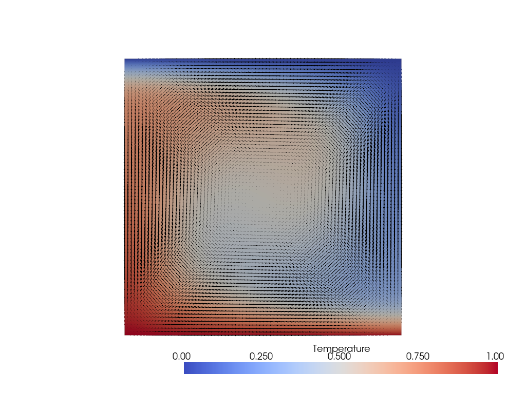
Here we can see a broad, high-temperature upwelling with a corresponding symmetric cold downwelling.
Case 1b#
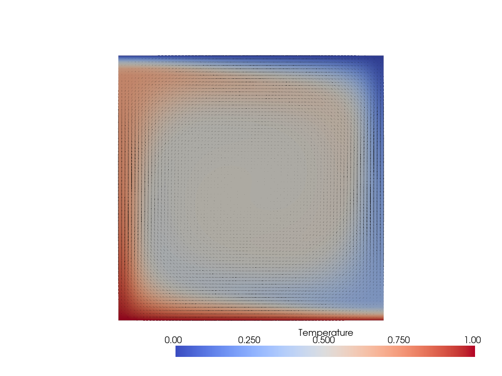
Case 1b is still isoviscous, using slightly higher vigor Ra \(=10^5\).
ne = 40
pp = 1
pT = 1
# Case 1b
Ra = 1.e5
v_1b, p_1b, T_1b = solve_blankenbach(Ra, ne, pp=pp, pT=pT)
T_1b.name = 'Temperature'
print('Nu = {}, vrms = {}'.format(*blankenbach_diagnostics(v_1b, T_1b)))
Iteration   Residual     Relative Residual
------------------------------------------
0           838.777      1
1           290.174      0.345949
2           122.083      0.145548
3           39.7105      0.0473434
4           12.8552      0.0153261
5           4.37539      0.0052164
6           1.44345      0.0017209
7           0.442106     0.000527084
8           0.124502     0.000148433
9           0.0322385    3.84351e-05
10          0.00787616   9.39005e-06
11          0.00198102   2.3618e-06
Nu = 9.701513273197865, vrms = 193.60002224124608
Again, the low resolution means our Nu value is inaccurate while our \(V_\text{rms}\) is close to the benchmark. Visualizing the solution we see a thinner upwelling and, still symmetric, downwelling.
# visualize
plotter_1b = fenics_sz.utils.plot.plot_scalar(T_1b, cmap='coolwarm', clim=[0,1])
fenics_sz.utils.plot.plot_vector_glyphs(v_1b, plotter=plotter_1b, color='k', factor=0.00005)
fenics_sz.utils.plot.plot_show(plotter_1b)
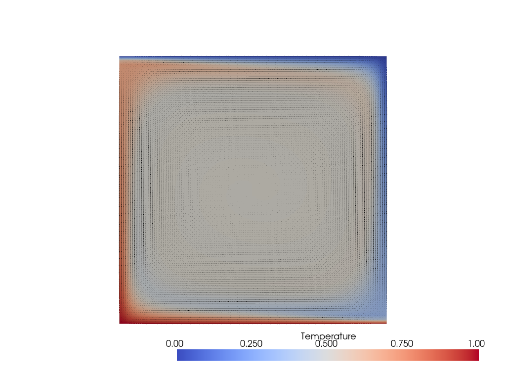
Case 1c#
Case 1c increase the Rayleigh number further to Ra \(=10^6\). This requires using higher resolution to resolve the boundary layers.
ne = 60
pp = 1
pT = 1
# Case 1c
Ra = 1.e6
v_1c, p_1c, T_1c = solve_blankenbach(Ra, ne, pp=pp, pT=pT)
T_1c.name = 'Temperature'
print('Nu = {}, vrms = {}'.format(*blankenbach_diagnostics(v_1c, T_1c)))
Iteration   Residual     Relative Residual
------------------------------------------
0           5607.35      1
1           2001.63      0.356965
2           836.783      0.14923
3           285.171      0.0508567
4           110.246      0.019661
5           44.6603      0.00796459
6           16.8674      0.0030081
7           5.71649      0.00101946
8           1.70737      0.000304487
9           0.446922     7.97029e-05
10          0.103398     1.84398e-05
11          0.0219308    3.91109e-06
Nu = 19.172102075792957, vrms = 836.5748453918482
We can see those thinner boundary features in the solution below.
# visualize
plotter_1c = fenics_sz.utils.plot.plot_scalar(T_1c, cmap='coolwarm', clim=[0,1])
fenics_sz.utils.plot.plot_vector_glyphs(v_1c, plotter=plotter_1c, color='k', factor=0.00001)
fenics_sz.utils.plot.plot_show(plotter_1c)
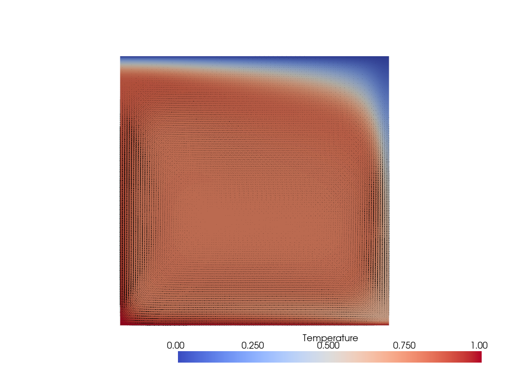
Case 2a#
Case 2a uses Ra \(=10^4\) but introduces a simple temperature dependent viscosity with a 1000-fold change in the viscosity across the domain (using \(\eta = e^{-b T}\) with \(b = \ln(10^3)\)).
ne = 60
pp = 1
pT = 1
# Case 2a
Ra = 1.e4
b = np.log(1.e3)
v_2a, p_2a, T_2a = solve_blankenbach(Ra, ne, pp=pp, pT=pT, b=b)
T_2a.name = 'Temperature'
print('Nu = {}, vrms = {}'.format(*blankenbach_diagnostics(v_2a, T_2a)))
Iteration   Residual     Relative Residual
------------------------------------------
0           56.0735      1
1           43.9069      0.783023
2           22.5086      0.401412
3           6.90407      0.123125
4           3.42584      0.0610955
5           2.45884      0.0438503
6           1.3469       0.0240203
7           0.640917     0.0114299
8           0.328306     0.00585491
9           0.177344     0.00316271
10          0.0879548    0.00156856
11          0.0402775    0.000718298
12          0.0250574    0.000446867
13          0.0208039    0.000371011
14          0.015428     0.000275139
15          0.00957477   0.000170754
16          0.00501916   8.95103e-05
17          0.0023052    4.11103e-05
18          0.00110446   1.96967e-05
19          0.000670147  1.19512e-05
20          0.000413838  7.38028e-06
21          0.000219495  3.91442e-06
Nu = 9.755711148057017, vrms = 482.1205639587135
Visualizing this solution we can see that the symmetry is gone with the upwelling now being much broader than the downwelling.
# visualize
plotter_2a = fenics_sz.utils.plot.plot_scalar(T_2a, cmap='coolwarm', clim=[0,1])
fenics_sz.utils.plot.plot_vector_glyphs(v_2a, plotter=plotter_2a, color='k', factor=0.00002)
fenics_sz.utils.plot.plot_show(plotter_2a)
Testing#
Error analysis#
Unlike in the previous cases, where we knew the analytical solution, here we do not. However we can still perform some rudimentary error analysis by comparing our solutions to the published values from other simulations and ensuring we are converging to the agreed upon benchmark solution. There is no guaranteed order of convergence in this analysis but, just like in the formal convergence tests performed on the previous cases, the trend should be towards decreasing error with increasing resolution.
We begin by noting the averaged extrapolated benchmark values from Wilson & van Keken (2023) (WvK in Table 2.5.1) as well as the relevant parameter values for each case.
values_wvk = {
    '1a': {'Nu': 4.88440907, 'vrms': 42.8649484},
    '1b': {'Nu': 10.53404, 'vrms': 193.21445},
    '1c': {'Nu': 21.97242, 'vrms': 833.9897},
    '2a': {'Nu': 10.06597, 'vrms': 480.4308},
    }
params = {
    '1a': {'Ra': 1.e4, 'b': None},
    '1b': {'Ra': 1.e5, 'b': None},
    '1c': {'Ra': 1.e6, 'b': None},
    '2a': {'Ra': 1.e4, 'b': np.log(1.e3)}
    }
Convergence test#
The benchmark values will be used in our evaluation of the errors in convergence_errors where we loop over the cases, polynomial orders (only of temperature here, pT), and numbers of elements (ne) comparing our diagnostic values to the published values.
def convergence_errors(pTs, nelements, cases, beta=1,
                       petsc_options_s=None, petsc_options_T=None,
                       attach_nullspace=False, attach_nearnullspace=True,
                       verbose=False, output_basename=None):
    """
    A python function to run a convergence test of a two-dimensional thermal
    convection problem in a unit square domain.
    Parameters:
    * pTs       - a list of temperature polynomial orders to test
    * nelements - a list of the number of elements to test
    * cases     - a list of benchmark cases to test (must be in ['1a', '1b', '1c', '2a'])
    * beta      - beta mesh refinement coefficient, < 1 refines the mesh at
                  the top and bottom boundaries (optional, defaults to  1, no refinement]
    * petsc_options_s - a dictionary of petsc options to pass to the Stokes solver
                      (optional, defaults to an LU direct solver using the MUMPS library)
    * petsc_options_T - a dictionary of petsc options to pass to the temperature solver
                      (optional, defaults to an LU direct solver using the MUMPS library)
    * attach_nullspace - flag indicating if the null space should be removed
                         iteratively rather than using a pressure reference point
                         (optional, defaults to False)
    * attach_nearnullspace - flag indicating if the preconditioner should be made
                             aware of the possible (near) nullspaces in the velocity
                             (optional, defaults to True)
    * verbose - print convergence information (optional, defaults to True)
    * output_basename - basename of file to write errors to (optional, defaults to no output)
    Returns:
    * errors - a dictionary of estimated errors with keys corresponding to the cases
    """

    errors = {}

    for case in cases:

        errors_Nu = []
        errors_vrms = []

        # get parameters
        params_c = params[case]
        Ra = params_c['Ra']
        b  = params_c['b']
        # get benchmark values
        values_c = values_wvk[case]
        Nu_e   = values_c['Nu']
        vrms_e = values_c['vrms']

        # Loop over the polynomial orders
        for pT in pTs:
            # Accumulate the values and errors
            Nus = []
            vrmss = []
            errors_Nu_pT   = []
            errors_vrms_pT = []
            # Loop over the resolutions
            for ne in nelements:
                # Solve the 2D Blankenbach thermal convection problem
                v_i, p_i, T_i = solve_blankenbach(Ra, ne, pp=1, pT=pT, b=b, beta=beta,
                                                  petsc_options_s=petsc_options_s,
                                                  petsc_options_T=petsc_options_T,
                                                  attach_nullspace=attach_nullspace,
                                                  attach_nearnullspace=attach_nearnullspace,
                                                  verbose=verbose)
                Nu, vrms = blankenbach_diagnostics(v_i, T_i)
                Nus.append(Nu)
                vrmss.append(vrms)
                Nuerr = np.abs(Nu - Nu_e)/Nu_e
                vrmserr = np.abs(vrms - vrms_e)/vrms_e
                errors_Nu_pT.append(Nuerr)
                errors_vrms_pT.append(vrmserr)
                # Print to screen and save if on rank 0
                if MPI.COMM_WORLD.rank == 0:
                    print('case={}, pT={}, ne={}, Nu={:.3f}, vrms={:.3f}, Nu err={:.3e}, vrms err={:.3e}'.format(case,pT,ne,Nu,vrms,Nuerr,vrmserr,))
            if MPI.COMM_WORLD.rank == 0:
                print('*************************************************')
            errors_Nu.append(errors_Nu_pT)
            errors_vrms.append(errors_vrms_pT)

            hs = 1./np.array(nelements)/pT

            # Write the errors to disk
            if MPI.COMM_WORLD.rank == 0:
                if output_basename is not None:
                    with open(str(output_basename) + '_case{}_pT{}.csv'.format(case, pT), 'w') as f:
                        np.savetxt(f, np.c_[nelements, hs, Nus, vrmss, errors_Nu, errors_vrms], delimiter=',',
                            header='nelements, hs, Nu, vrms, Nu_err, vrms_err')

        errors[case] = (errors_Nu, errors_vrms)

    return errors
Running this function on all cases we can see that our errors are (for the most part) decreasing.
cases = ['1a', '1b', '1c', '2a']
# List of polynomial orders to try
pTs = [1]
# List of resolutions to try
nelements = [32, 64, 128]

errors = convergence_errors(pTs, nelements, cases)
case=1a, pT=1, ne=32, Nu=4.672, vrms=42.913, Nu err=4.356e-02, vrms err=1.126e-03
case=1a, pT=1, ne=64, Nu=4.801, vrms=42.877, Nu err=1.707e-02, vrms err=2.840e-04
case=1a, pT=1, ne=128, Nu=4.849, vrms=42.868, Nu err=7.269e-03, vrms err=7.084e-05
*************************************************
case=1b, pT=1, ne=32, Nu=9.367, vrms=193.803, Nu err=1.108e-01, vrms err=3.044e-03
case=1b, pT=1, ne=64, Nu=10.135, vrms=193.368, Nu err=3.792e-02, vrms err=7.972e-04
case=1b, pT=1, ne=128, Nu=10.395, vrms=193.253, Nu err=1.317e-02, vrms err=2.010e-04
*************************************************
case=1c, pT=1, ne=32, Nu=15.699, vrms=839.829, Nu err=2.855e-01, vrms err=7.002e-03
case=1c, pT=1, ne=64, Nu=19.427, vrms=836.286, Nu err=1.158e-01, vrms err=2.754e-03
case=1c, pT=1, ne=128, Nu=21.138, vrms=834.591, Nu err=3.796e-02, vrms err=7.211e-04
*************************************************
case=2a, pT=1, ne=32, Nu=9.333, vrms=481.928, Nu err=7.281e-02, vrms err=3.116e-03
case=2a, pT=1, ne=64, Nu=9.783, vrms=481.974, Nu err=2.809e-02, vrms err=3.213e-03
case=2a, pT=1, ne=128, Nu=9.960, vrms=480.883, Nu err=1.048e-02, vrms err=9.418e-04
*************************************************
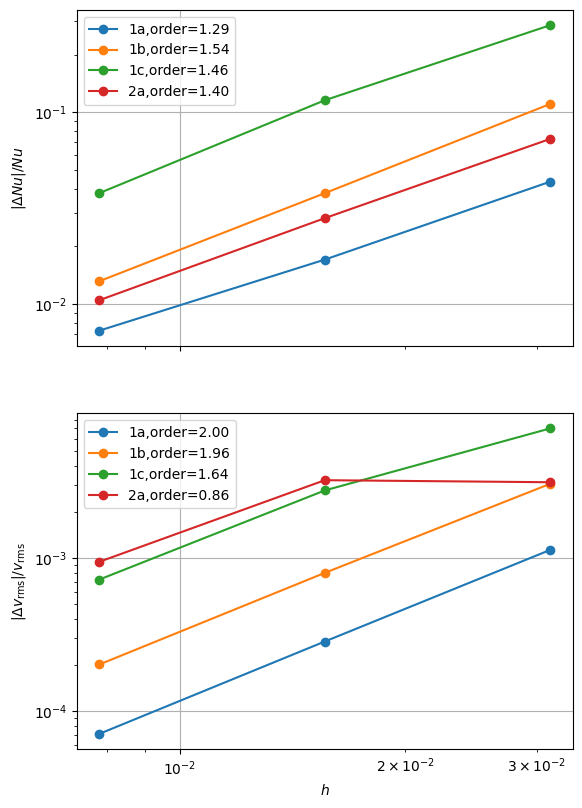
As before, this is easiest to see by plotting the errors and fitting an estimated convergence order to them using the function plot_convergence.
def plot_convergence(pTs, nelements, errors, output_filename=None):
    """
    A python function to plot convergence of the given errors.
    Parameters:
    * pTs             - a list of temperature polynomial orders to test
    * nelements       - a list of the number of elements to test
    * errors          - errors dictionary (keys per case) from convergence_errors
    * output_filename - filename for output plot (optional, defaults to no output)
    Returns:
    * fits            - a dictionary (keys per case) of convergence order fits
    """
    # Open a figure for plotting
    if MPI.COMM_WORLD.rank == 0:
        fig, (axNu, axvrms) = pl.subplots(nrows=2, figsize=(6.4,9.6), sharex=True)

    fits = {}

    for case, (errors_Nu, errors_vrms) in errors.items():
        fits_Nu_p = []
        fits_vrms_p = []
        # Loop over the polynomial orders
        for i, pT in enumerate(pTs):
            # Work out the order of convergence at this pT
            hs = 1./np.array(nelements)/pT

            # Fit a line to the convergence data
            fitNu = np.polyfit(np.log(hs), np.log(errors_Nu[i]),1)
            fitvrms = np.polyfit(np.log(hs), np.log(errors_vrms[i]),1)

            fits_Nu_p.append(float(fitNu[0]))
            fits_vrms_p.append(float(fitvrms[0]))
            if MPI.COMM_WORLD.rank == 0:
                print("case {} order of accuracy pT={}, Nu order={}, vrms order={}".format(case, pT, fitNu[0], fitvrms[0]))

                # log-log plot of the error
                label = '{}'.format(case,)
                if len(pTs) > 1: label = label+',pT={}'.format(pT,)
                axNu.loglog(hs, errors_Nu[i], 'o-', label=label+',order={:.2f}'.format(fitNu[0],))
                axvrms.loglog(hs, errors_vrms[i], 'o-', label=label+',order={:.2f}'.format(fitvrms[0],))
        fits[case] = (fits_Nu_p, fits_vrms_p)

    if MPI.COMM_WORLD.rank == 0:
        # Tidy up the plot
        axNu.set_ylabel('$|\\Delta Nu|/Nu$')
        axNu.grid()
        axNu.legend()
        axvrms.set_xlabel('$h$')
        axvrms.set_ylabel('$|\\Delta v_\\text{rms}|/v_\\text{rms}$')
        axvrms.grid()
        axvrms.legend()

        # Write convergence to disk
        if output_filename is not None:
            fig.savefig(output_filename)
            print("***********  convergence figure in "+str(output_filename))

    return fits
fits = plot_convergence(pTs, nelements, errors, output_filename=output_folder / "blankenbach_convergence.png")
case 1a order of accuracy pT=1, Nu order=1.2915710919471073, vrms order=1.9954422964136325
case 1b order of accuracy pT=1, Nu order=1.5363677716431217, vrms order=1.9601287254918287
case 1c order of accuracy pT=1, Nu order=1.4555229836604044, vrms order=1.6397555168848175
case 2a order of accuracy pT=1, Nu order=1.3981332540094622, vrms order=0.8629793144331601
*********** convergence figure in output/blankenbach_convergence.png
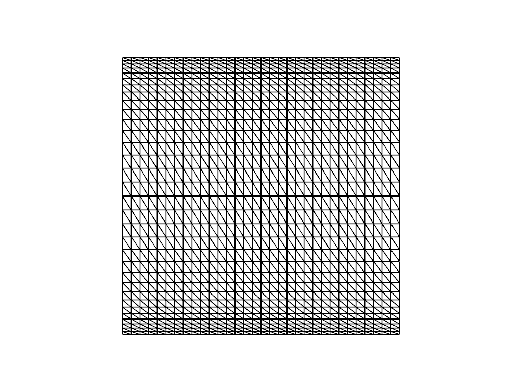
As some of the resulting estimated orders of convergence are quite low we can try improving the solution by refining the mesh near the top and bottom of the domain using the parameter beta. For example for a low resolution mesh ne = 32 this looks like
ne = 32
beta = 0.2
mesh = transfinite_unit_square_mesh(ne, ne, beta=beta)
plotter_beta = fenics_sz.utils.plot.plot_mesh(mesh, gather=True, show_edges=True, style="wireframe", color='k', line_width=2)
fenics_sz.utils.plot.plot_show(plotter_beta)
Rerunning the convergence test with beta = 0.2
errors_beta = convergence_errors(pTs, nelements, cases, beta=beta)
fits_beta = plot_convergence(pTs, nelements, errors_beta, output_filename=output_folder / "blankenbach_convergence_beta.png")
case=1a, pT=1, ne=32, Nu=4.759, vrms=42.899, Nu err=2.566e-02, vrms err=8.020e-04
case=1a, pT=1, ne=64, Nu=4.824, vrms=42.874, Nu err=1.232e-02, vrms err=2.010e-04
case=1a, pT=1, ne=128, Nu=4.855, vrms=42.867, Nu err=6.058e-03, vrms err=4.998e-05
*************************************************
case=1b, pT=1, ne=32, Nu=10.114, vrms=193.219, Nu err=3.984e-02, vrms err=2.428e-05
case=1b, pT=1, ne=64, Nu=10.358, vrms=193.214, Nu err=1.667e-02, vrms err=4.412e-06
case=1b, pT=1, ne=128, Nu=10.455, vrms=193.214, Nu err=7.543e-03, vrms err=1.959e-06
*************************************************
case=1c, pT=1, ne=32, Nu=20.009, vrms=832.606, Nu err=8.935e-02, vrms err=1.659e-03
case=1c, pT=1, ne=64, Nu=21.272, vrms=833.397, Nu err=3.190e-02, vrms err=7.103e-04
case=1c, pT=1, ne=128, Nu=21.708, vrms=833.827, Nu err=1.205e-02, vrms err=1.951e-04
*************************************************
case=2a, pT=1, ne=32, Nu=9.651, vrms=478.090, Nu err=4.118e-02, vrms err=4.871e-03
case=2a, pT=1, ne=64, Nu=9.892, vrms=479.784, Nu err=1.730e-02, vrms err=1.345e-03
case=2a, pT=1, ne=128, Nu=9.990, vrms=480.266, Nu err=7.565e-03, vrms err=3.430e-04
*************************************************
case 1a order of accuracy pT=1, Nu order=1.0413301819976803, vrms order=2.002046087517078
case 1b order of accuracy pT=1, Nu order=1.2005602816556635, vrms order=1.8156599675883764
case 1c order of accuracy pT=1, Nu order=1.4450500656028138, vrms order=1.5437494333391681
case 2a order of accuracy pT=1, Nu order=1.222284020164673, vrms order=1.9139183170874132
*********** convergence figure in output/blankenbach_convergence_beta.png
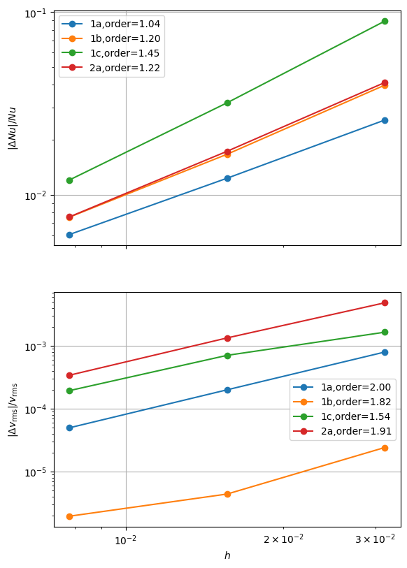
We see some improvements in the convergence and can put a simple test that these solutions should converge at at least first order.
assert(all(fit > 1.0 for fits_p in fits_beta.values() for fits in fits_p for fit in fits))
In the next notebook we will test that this convergence behavior is maintained in parallel and also examine the performance of our implementation.