Batchelor Cornerflow Example

Author: Cian Wilson

Description

As a reminder we are seeking the approximate velocity and pressure solution of the Stokes equation

(57)\[\begin{align} -\nabla\cdot \left(\frac{\nabla\tilde{\vec{v}} + \nabla\tilde{\vec{v}}^T}{2}\right) + \nabla \tilde{P} &= 0 && \text{in }\Omega \\ \nabla\cdot\tilde{\vec{v}} &= 0 && \text{in }\Omega \end{align}\]

in a unit square domain, \(\Omega = [0,1]\times[0,1]\).

We apply strong Dirichlet boundary conditions for velocity on all four boundaries

(58)\[\begin{align} \tilde{\vec{v}} &= (0,0)^T && \text{on } \partial\Omega \text{ where } x=0 \\ \tilde{\vec{v}} &= (U, 0)^T && \text{on } \partial\Omega \text{ where } y=0 \\ \tilde{\vec{v}} &= \vec{v} && \text{on } \partial\Omega \text{ where } x=1 \text{ or } y = 1 \end{align}\]

and a constraint on the pressure to remove its null space, e.g. by applying a reference point

(59)\[\begin{align} P &= 0 && \text{at } (x, y) = (0,0) \end{align}\]

Parallel Scaling

In the previous notebook we tested that the error in our implementation of a Batchelor corner-flow problem in two-dimensions converged as the number of elements increased and found suboptimal results owing to the discontinuous boundary conditions imposed in this problem. We also wish to test for parallel scaling of this problem, assessing if the simulation wall time decreases as the number of processors used to solve it is increases.

Here we perform strong scaling tests on our function solve_batchelor from notebooks/02_background/2.4b_batchelor.ipynb. As we will see this is more challenging than in the 2D Poisson case as the solution algorithm must deal with the pressure null space and the fact that we are seeking the solution to a saddle-point problem with a zero diagonal block.

Preamble

We start by loading all the modules we will require.

import sys, os
basedir = ''
if "__file__" in globals(): basedir = os.path.dirname(__file__)
path = os.path.join(basedir, os.path.pardir, os.path.pardir, 'python')
sys.path.append(path)
import utils.ipp
from background.batchelor import test_plot_convergence
import pathlib
output_folder = pathlib.Path(os.path.join(basedir, "output"))
output_folder.mkdir(exist_ok=True, parents=True)

Implementation

We perform the strong parallel scaling test using a utility function (from python/utils/ipp.py) that loops over a list of the number of processors calling our function for a given number of elements, ne, and polynomial order p. It runs our function solve_batchelor a specified number of times and evaluates and returns the time taken for each of a number of requested steps.

# the list of the number of processors we will use
nprocs_scale = [1, 2, 4]

# the number of elements to solve the problem on
ne = 128

# the polynomial degree of our pressure field
p = 1

# perform the calculation a set number of times
number = 1

# We are interested in the time to create the mesh,
# declare the functions, assemble the problem and solve it.
# From our implementation in `solve_poisson_2d` it is also
# possible to request the time to declare the Dirichlet and
# Neumann boundary conditions and the forms.
steps = [
          'Mesh', 'Function spaces',
          'Assemble', 'Solve',
         ]

# declare a dictionary to store the times each step takes
maxtimes = {}

Direct

To start with we test the scaling with the default solver options, which is a direct LU decomposition using the MUMPS library implementation.

maxtimes['Direct'] = utils.ipp.profile_parallel(nprocs_scale, steps, path, 'background.batchelor', 'solve_batchelor', 
                                                ne, p, number=number,
                                                output_filename=output_folder / 'batchelor_scaling_direct_block.png')

=========================
                 1           2           4           
Mesh             0.02        0.04        0.06        
Function spaces  0.02        0.01        0.01        
Assemble         0.28        0.16        0.14        
Solve            1.48        1.27        1.41        
=========================

***********  profiling figure in output/batchelor_scaling_direct_block.png

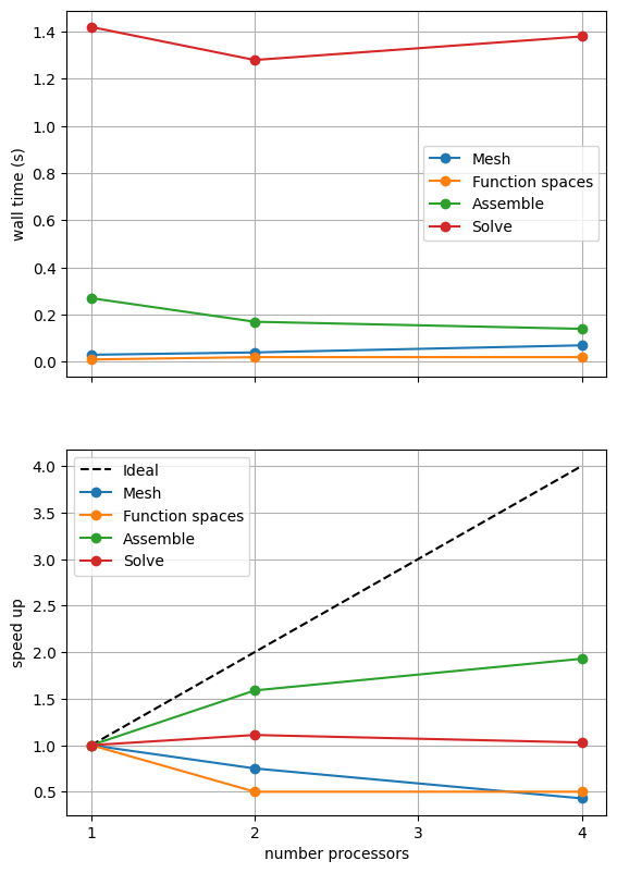
“Speed up” is defined as the wall time on a given number of processors divided by the wall time on the smallest number of processors. Ideally this should increase linearly with the number of processors with slope 1. Such ideal scaling is rarely realized due to factors like the increasing costs of communication between processors but the behavior of the scaling test will also strongly depend on the computational resources available on the machine where this notebook is run. In particular when the website is generated it has to run as quickly as possible on github, hence we limit our requested numbers of processors, size of the problem (ne and p) and number of calculations to average over (number) in the default setup of this notebook.

For comparison we provide the output of this notebook using ne = 256, p = 1 and number = 10 in Figure 2.4.2 generated on a dedicated machine using a local conda installation of the software.

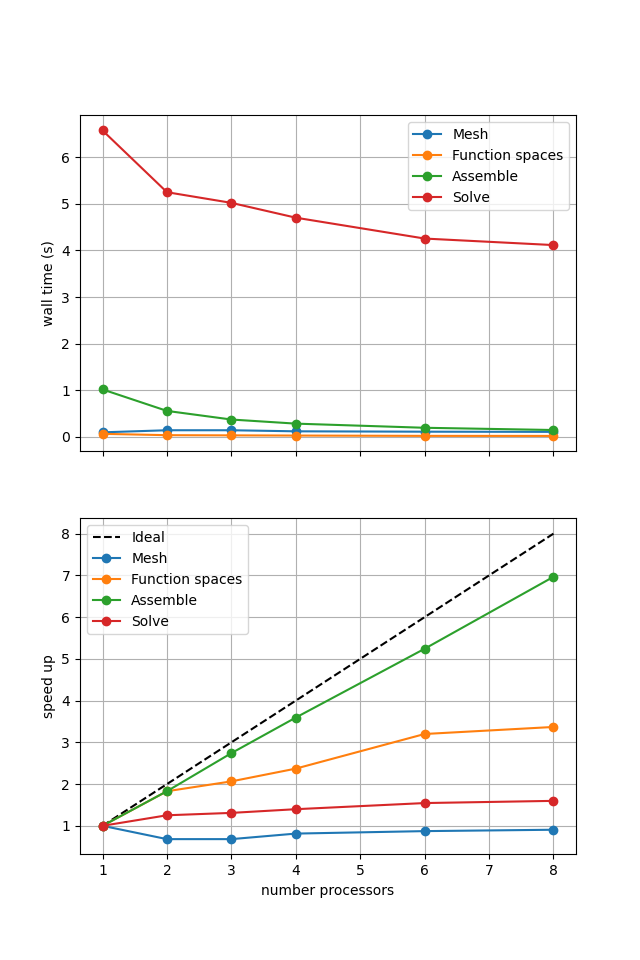
Figure 2.4.2 Scaling results for a direct solver with ne = 256, p = 1 averaged over number = 10 calculations using a local conda installation of the software on a dedicated machine.

As in the Poisson 2D case we can see that assembly and function space declarations scale well, with assembly being almost ideal. However meshing and the solve barely scale at all. The meshing takes place on a single process before being communicated to the other processors, hence we do not expect this step to scale. Additionally the cost (wall time taken) of meshing is so small that it is not a significant factor in these simulations. However the solution step is our most significant cost and would ideally scale. Its failure to do so here is a result of an initial analysis step that is performed in serial (on a single processor), the significance of which will decrease once the solver is used more than once per simulation.

Switching to alternative solvers is not as simple for the Stokes system as it was in the Poisson 2D example. We need to modify our implementation because

1. we are solving a saddle point system with a zero pressure block in the matrix

2. each block (for the velocity and pressure) of the matrix would ideally be preconditioned differently to get the best iterative solver convergence behavior

3. our solver must be able to deal with the pressure null space

We will try this in the next notebook but first we will check that the solution using a direct solver is still converging in parallel. We do this by running our convergence test from notebooks/02_background/2.4b_batchelor.ipynb in parallel using the utility function utils.ipp.run_parallel.

# the list of the number of processors to test the convergence on
nprocs_conv = [2,]
# List of polynomial orders to try
ps = [1, 2]
# List of resolutions to try
nelements = [10, 20, 40, 80]

errors_l2_all = utils.ipp.run_parallel(nprocs_conv, path, 'background.batchelor', 'convergence_errors', ps, nelements)

for errors_l2 in errors_l2_all:
    test_passes = test_plot_convergence(ps, nelements, errors_l2)
    assert(test_passes)

order of accuracy p=1, order=1.0000050785210919
order of accuracy p=2, order=0.9999999771173622

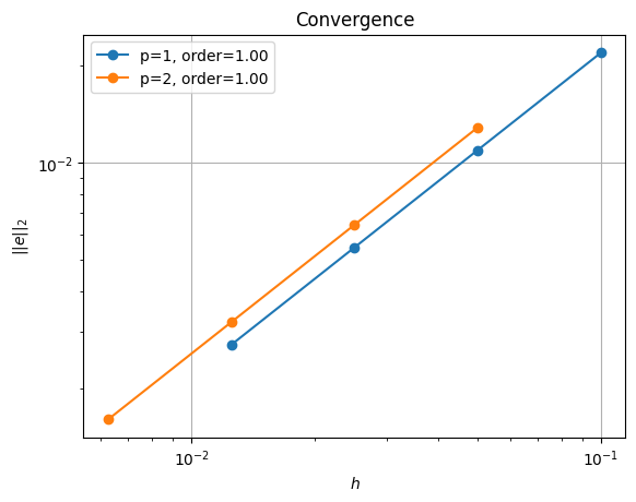
We can see that, even in parallel, we reproduce the (suboptimal) convergence of the problem in serial.