Subduction Zone Model Setup#
Implementation#
As a reminder our implementation is following a similar workflow to that seen in the background examples.
we will describe the subduction zone geometry and tesselate it into non-overlapping triangles to create a mesh
we will declare function spaces for the temperature, wedge velocity and pressure, and slab velocity and pressure
using these function spaces we will declare trial and test functions
we will define Dirichlet boundary conditions at the boundaries as described in the introduction
we will describe discrete weak forms for temperature and each of the coupled velocity-pressure systems that will be used to assemble the matrices (and vectors) to be solved
we will set up matrices and solvers for the discrete systems of equations
we will solve the matrix problems
In the previous two notebooks we have only tackled step 1. Steps 2-4 will be implemented in this notebook before implementing the equations and solvers in subsequent notebooks. Here we are going to start a base BaseSubductionProblem python class that will take in the subduction zone geometry object we can now create using create_sz_geometry and use it to set up finite element function spaces and apply appropriate boundary conditions to the resulting finite element functions (steps 2-4). In subsequent notebooks we will describe the mathematical problems we wish to solve and provide finite element forms to the class to solve (step 5). These will depend on the rheology and time-dependence we assume and each case will be implemented in a separate notebook. In the benchmark section we will demonstrate our steady-state implementation using benchmark cases 1 & 2 from Wilson & van Keken, PEPS, 2023 (II), where case 1 uses a simple isoviscous rheology and case 2 uses a dislocation creep viscosity.
Preamble#
Let’s start by adding the path to the modules in the python folder to the system path (so we can find the our custom modules).
import sys, os
basedir = ''
if "__file__" in globals(): basedir = os.path.dirname(__file__)
sys.path.insert(0, os.path.join(basedir, os.path.pardir, os.path.pardir, 'python'))
Let’s also load the module generated by the previous notebooks to get access to the parameters and functions defined there.
from fenics_sz.sz_problems.sz_params import default_params, allsz_params
from fenics_sz.sz_problems.sz_slab import create_slab
from fenics_sz.sz_problems.sz_geometry import create_sz_geometry
Then let’s load all the required modules at the beginning.
import fenics_sz.utils
import dolfinx as df
import numpy as np
import scipy as sp
import ufl
import basix.ufl as bu
import pathlib
output_folder = pathlib.Path(os.path.join(basedir, "output"))
output_folder.mkdir(exist_ok=True, parents=True)
BaseSubductionProblem class#
To build the python class in an parseable way we will be using some python trickery, rederiving the class in each cell, which isn’t really how this would be done outside of a jupyter notebook but here it allows us to annotate what we are doing as we progress through the steps above.
We begin by declaring the class and its members. Those initialized to None need to be initialized in the class routines that we will describe in the following cells. Others are initialized to appropriate default values. Only the first few are intended to be modified and we will write functions to allow us to do this later.
For now this cell is mostly bookkeeping but it does allow us to anticipate what the functions we write subsequently will have access to once this class is properly initialized.
class BaseSubductionProblem:
    """
    A class describing a kinematic slab subduction zone thermal problem.
    """

    def members(self):
        # geometry object
        self.geom = None

        # case specific
        self.A      = None      # age of subducting slab (Myr)
        self.Vs     = None      # slab speed (mm/yr)
        self.sztype = None      # type of sz ('continental' or 'oceanic')
        self.Ac     = None      # age of overriding plate (Myr) - oceanic only
        self.As     = None      # age of subduction (Myr) - oceanic only
        self.qs     = None      # surface heat flux (W/m^2) - continental only

        # non-dim parameters
        self.Ts      = 0.0       # surface temperature (non-dim, also deg C)
        self.Tm      = 1350.0    # mantle temperature (non-dim, also deg C)
        self.kc      = 0.8064516 # crustal thermal conductivity (non-dim) - continental only
        self.km      = 1.0       # mantle thermal conductivity (non-dim)
        self.rhoc    = 0.8333333 # crustal density (non-dim) - continental only
        self.rhom    = 1.0       # mantle density (non-dim)
        self.cp      = 1.0       # heat capacity (non-dim)
        self.H1      = 0.419354  # upper crustal volumetric heat production (non-dim) - continental only
        self.H2      = 0.087097  # lower crustal volumetric heat production (non-dim) - continental only

        # dislocation creep parameters
        self.etamax = 1.0e25    # maximum viscosity (Pa s)
        self.nsigma = 3.5       # stress viscosity power law exponent (non-dim)
        self.Aeta   = 28968.6   # pre-exponential viscosity constant (Pa s^(1/nsigma))
        self.E      = 540.0e3   # viscosity activation energy (J/mol)

        # finite element degrees
        self.p_p = 1  # pressure
        self.p_T = 2  # temperature

        # mesh options
        self.partition_by_region = True # partition the mesh by region or not

        # only allow these options to be set from the update and __init__ functions
        self.allowed_input_parameters = ['A', 'Vs', 'sztype', 'Ac', 'As', 'qs', \
                                         'Ts', 'Tm', 'km', 'rhom', 'cp', \
                                         'etamax', 'nsigma', 'Aeta', 'E', \
                                         'p_p', 'p_T', 'partition_by_region']
        self.allowed_if_continental   = ['kc', 'rhoc', 'H1', 'H2']

        self.required_parameters     = ['A', 'Vs', 'sztype']
        self.required_if_continental = ['qs']
        self.required_if_oceanic     = ['Ac', 'As']

        # reference values
        self.k0     = 3.1       # reference thermal conductivity (W/m/K)
        self.rho0   = 3300.0    # reference density (kg/m^3)
        self.cp0    = 1250.0    # reference heat capacity (J/kg/K)
        self.h0     = 1000.0    # reference length scale (m)
        self.eta0   = 1.0e21    # reference viscosity (Pa s)
        self.T0     = 1.0       # reference temperature (K)
        self.R      = 8.3145    # gas constant (J/mol/K)

        # derived reference values
        self.kappa0 = None  # reference thermal diffusivity (m^2/s)
        self.v0     = None  # reference velocity (m/s)
        self.t0     = None  # reference time-scale (s)
        self.e0     = None  # reference strain rate (/s)
        self.p0     = None  # reference pressure (Pa)
        self.H0     = None  # reference heat source (W/m^3)
        self.q0     = None  # reference heat flux (W/m^2)

        # derived parameters
        self.A_si   = None  # age of subducting slab (s)
        self.Vs_nd  = None  # slab speed (non-dim)
        self.Ac_si  = None  # age of overriding plate (s) - oceanic only
        self.As_si  = None  # age of subduction (s) - oceanic only
        self.qs_nd  = None  # surface heat flux (non-dim) - continental only

        # derived from the geometry object
        self.deltaztrench = None
        self.deltaxcoast  = None
        self.deltazuc     = None
        self.deltazc      = None

        # mesh related
        self.mesh       = None
        self.cell_tags  = None
        self.facet_tags = None

        # MPI communicator
        self.comm       = None

        # dimensions and mesh statistics
        self.gdim = None
        self.tdim = None
        self.fdim = None

        # region ids
        self.wedge_rids       = None
        self.slab_rids        = None
        self.crust_rids       = None

        # wedge submesh
        self.wedge_submesh    = None
        self.wedge_cell_tags  = None
        self.wedge_facet_tags = None
        self.wedge_cell_map   = None
        self.wedge_rank       = True

        # slab submesh
        self.slab_submesh    = None
        self.slab_cell_tags  = None
        self.slab_facet_tags = None
        self.slab_cell_map   = None
        self.slab_rank       = True

        # integral measures
        self.dx = None
        self.wedge_ds = None

        # function spaces
        self.Vslab_v  = None
        self.Vslab_p  = None
        self.Vwedge_v = None
        self.Vwedge_p = None
        self.V_T      = None

        # FE functions
        self.slab_vs_i  = None
        self.slab_ps_i  = None
        self.wedge_vw_i = None
        self.wedge_pw_i = None
        self.T_i         = None
        self.T_n         = None

        # Functions that need interpolation
        self.vs_i      = None
        self.ps_i      = None
        self.vw_i      = None
        self.pw_i      = None
        self.slab_T_i  = None
        self.wedge_T_i = None

        # test functions
        self.slab_vs_t  = None
        self.slab_ps_t  = None
        self.wedge_vw_t = None
        self.wedge_pw_t = None
        self.T_t        = None

        # trial functions
        self.slab_vs_a  = None
        self.slab_ps_a  = None
        self.wedge_vw_a = None
        self.wedge_pw_a = None
        self.T_a        = None

        # boundary conditions
        self.bcs_T   = None # temperature
        self.bcs_vw = None  # wedge velocity
        self.bcs_vs = None  # slab velocity
1. Mesh#
Just as in simpler problems our first step is to initialize the mesh. We do this just as we did in the previous notebooks, through the geometry object that we assume is initialized by create_sz_geometry and is now available as a member of the class (we will initialize this later).
Here describing the geometry is further complicated by the fact that we will want to solve three problems:
a thermal problem across the whole domain (the slab, the mantle wedge and the crust)
a mechanical Stokes problem for the flow in the slab (just in the slab portion of the domain, beneath the slab surface)
a mechanical Stokes problem for the corner flow in the mantle wedge (just in the mantle wedge portion of the domain, above the slab surface)
Note that we do not solve the Stokes equations in the crust, which is assumed rigid (zero velocity).
To facilitate these three problems we create:
a mesh of the whole domain (for the thermal problem)
and extract from it:
a submesh of the slab, and
a submesh of the mantle wedge.
We also record various other pieces of information about the mesh, tags demarking different regions and boundaries, and maps to and from the submeshes.
class BaseSubductionProblem(BaseSubductionProblem):
    def setup_meshes(self):
        """
        Generate the mesh from the supplied geometry then extract submeshes representing
        the wedge and slab for the Stokes problems in these regions.
        """
        # check we have a geometry object attached
        assert(self.geom is not None)

        with df.common.Timer("Mesh"):
            # generate the mesh using gmsh
            # this command also returns cell and facets tags identifying regions and boundaries in the mesh
            self.mesh, self.cell_tags, self.facet_tags = self.geom.generatemesh(partition_by_region=self.partition_by_region)
            self.comm = self.mesh.comm

            # record the dimensions
            self.gdim = self.mesh.geometry.dim
            self.tdim = self.mesh.topology.dim
            self.fdim = self.tdim - 1

            # record the region ids for the wedge, slab and crust based on the geometry
            self.wedge_rids = tuple(set([v['rid'] for k,v in self.geom.wedge_dividers.items()]+[self.geom.wedge_rid]))
            self.slab_rids  = tuple([self.geom.slab_rid])
            self.crust_rids = tuple(set([v['rid'] for k,v in self.geom.crustal_layers.items()]))

            # generate the wedge submesh
            # this command also returns cell and facet tags mapped from the parent mesh to the submesh
            # additionally a cell map maps cells in the submesh to the parent mesh
            self.wedge_submesh, self.wedge_cell_tags, self.wedge_facet_tags, self.wedge_cell_map = \
                                fenics_sz.utils.mesh.create_submesh(self.mesh,
                                                    np.concatenate([self.cell_tags.find(rid) for rid in self.wedge_rids]), \
                                                    self.cell_tags, self.facet_tags, split_comm=self.partition_by_region)
            # record whether this MPI rank has slab DOFs or not
            self.wedge_rank = (not self.partition_by_region) or (self.wedge_submesh.topology.index_map(self.tdim).size_local > 0)

            # generate the slab submesh
            # this command also returns cell and facet tags mapped from the parent mesh to the submesh
            # additionally a cell map maps cells in the submesh to the parent mesh
            self.slab_submesh, self.slab_cell_tags, self.slab_facet_tags, self.slab_cell_map  = \
                                fenics_sz.utils.mesh.create_submesh(self.mesh,
                                                    np.concatenate([self.cell_tags.find(rid) for rid in self.slab_rids]), \
                                                    self.cell_tags, self.facet_tags, split_comm=self.partition_by_region)
            # record whether this MPI rank has wedge DOFs or not
            self.slab_rank = (not self.partition_by_region) or (self.slab_submesh.topology.index_map(self.tdim).size_local > 0)

            # set up UFL measures that know about the cell and facet tags
            self.dx = ufl.Measure("dx", domain=self.mesh, subdomain_data=self.cell_tags)
            self.wedge_ds = ufl.Measure("ds", domain=self.wedge_submesh, subdomain_data=self.wedge_facet_tags)
2-3. Function spaces & functions#
With a mesh in hand we can initialize the functionspaces and dolfinx Functions representing finite element functions that we will use to solve our problem.
We are going to be solving problems for:
velocity and pressure in the wedge
velocity and pressure in the slab
temperature in the full domain
and need to select appropriate finite elements for each. We’re going to use continuous “Lagrange” elements for all finite element functions but the degree of the polynomials for velocity and pressure cannot be chosen independently and instead need to be selected as an appropriate mixed element pair for numerical stability reasons. We’re going to use a “Taylor-Hood” element pair, where the velocity degree is one higher than the pressure so only the pressure degree (p_p) can be set independently (and defaults to 1 so by default our element pair is known as P2P1). The temperature degree (p_T) can be set independently but a reasonable default is 2.
With appropriate finite elements selected we can declare function spaces, test, trial and solution finite element functions on the various meshes. Because our temperature problem will need access to the velocity and pressure from the submeshes, and vice versa, we declare multiple versions of each function on each sub and parent mesh and will later use them to interpolate the values between the domains.
class BaseSubductionProblem(BaseSubductionProblem):
    def setup_functionspaces(self):
        """
        Set up the functionspaces for the problem.
        """

        with df.common.Timer("Functions Stokes"):
            # create finite elements for velocity and pressure
            # use a P2P1 (Taylor-Hood) element pair where the velocity
            # degree is one higher than the pressure (so only the pressure
            # degree can be set)
            v_e = bu.element("Lagrange", self.mesh.basix_cell(), self.p_p+1, shape=(self.gdim,), dtype=df.default_real_type)
            p_e = bu.element("Lagrange", self.mesh.basix_cell(), self.p_p, dtype=df.default_real_type)

            def create_vp_functions(mesh, name_prefix):
                """
                Create velocity and pressure functions
                """
                # set up the velocity and pressure function spaces
                V_v, V_p = df.fem.functionspace(mesh, v_e), df.fem.functionspace(mesh, p_e)

                # Set up the velocity and pressure functions
                v_i, p_i = df.fem.Function(V_v), df.fem.Function(V_p)
                v_i.name = name_prefix+"v"
                p_i.name = name_prefix+"p"
                # set up the mixed velocity, pressure test function
                v_t, p_t = ufl.TestFunction(V_v), ufl.TestFunction(V_p)
                # set up the mixed velocity, pressure trial function
                v_a, p_a = ufl.TrialFunction(V_v), ufl.TrialFunction(V_p)

                # return everything
                return V_v, V_p, v_i, p_i, v_t, p_t, v_a, p_a

            # set up slab functionspace, collapsed velocity sub-functionspace,
            # combined velocity-pressure Function, split velocity and pressure Functions,
            # and trial and test functions for
            # 1. the slab submesh
            self.Vslab_v, self.Vslab_p, \
                        self.slab_vs_i, self.slab_ps_i, \
                        self.slab_vs_t, self.slab_ps_t, \
                        self.slab_vs_a, self.slab_ps_a = create_vp_functions(self.slab_submesh, "slab_")

            # 2. the wedge submesh
            self.Vwedge_v, self.Vwedge_p, \
                        self.wedge_vw_i, self.wedge_pw_i, \
                        self.wedge_vw_t, self.wedge_pw_t, \
                        self.wedge_vw_a, self.wedge_pw_a = create_vp_functions(self.wedge_submesh, "wedge_")

            # set up the velocity and pressure functionspace (not stored)
            V_v, V_p = df.fem.functionspace(self.mesh, v_e), df.fem.functionspace(self.mesh, p_e)

            # set up functions defined on the whole mesh
            # to interpolate the wedge and slab velocities
            # and pressures to
            self.vs_i = df.fem.Function(V_v)
            self.vs_i.name = "vs"
            self.ps_i = df.fem.Function(V_p)
            self.ps_i.name = "ps"
            self.vw_i = df.fem.Function(V_v)
            self.vw_i.name = "vw"
            self.pw_i = df.fem.Function(V_p)
            self.pw_i.name = "pw"

        with df.common.Timer("Functions Temperature"):
            # temperature element
            # the degree of the element can be set independently through p_T
            T_e = bu.element("Lagrange", self.mesh.basix_cell(), self.p_T, dtype=df.default_real_type)
            # and functionspace on the overall mesh
            self.V_T  = df.fem.functionspace(self.mesh, T_e)

            # create a dolfinx Function for the temperature
            self.T_i = df.fem.Function(self.V_T)
            self.T_i.name = "T"
            self.T_n = df.fem.Function(self.V_T)
            self.T_n.name = "T_n"
            self.T_t = ufl.TestFunction(self.V_T)
            self.T_a = ufl.TrialFunction(self.V_T)

            # on the slab submesh
            Vslab_T = df.fem.functionspace(self.slab_submesh, T_e)
            # and on the wedge submesh
            Vwedge_T = df.fem.functionspace(self.wedge_submesh, T_e)
            # set up Functions so the solution can be interpolated to these subdomains
            self.slab_T_i  = df.fem.Function(Vslab_T)
            self.slab_T_i.name = "slab_T"
            self.wedge_T_i = df.fem.Function(Vwedge_T)
            self.wedge_T_i.name = "wedge_T"
Since we’ve just declared multiple Functions on multiple domains, let’s set up some convenience python functions to perform the interpolations:
from the global temperature to the temperature declared in the slab and wedge
from the slab and wedge velocities to global versions of each
from the slab and wedge pressures to the global versions of each
class BaseSubductionProblem(BaseSubductionProblem):
    def update_T_functions(self):
        """
        Update the temperature functions defined on the submeshes, given a solution on the full mesh.
        """
        with df.common.Timer("Interpolate Temperature"):
            self.slab_T_i.interpolate(self.T_i, cells0=self.slab_cell_map, cells1=np.arange(len(self.slab_cell_map)))
            self.wedge_T_i.interpolate(self.T_i, cells0=self.wedge_cell_map, cells1=np.arange(len(self.wedge_cell_map)))

    def update_v_functions(self):
        """
        Update the velocity functions defined on the full mesh, given solutions on the sub meshes.
        """
        with df.common.Timer("Interpolate Stokes"):
            self.vs_i.interpolate(self.slab_vs_i, cells0=np.arange(len(self.slab_cell_map)), cells1=self.slab_cell_map)
            self.vw_i.interpolate(self.wedge_vw_i, cells0=np.arange(len(self.wedge_cell_map)), cells1=self.wedge_cell_map)

    def update_p_functions(self):
        """
        Update the pressure functions defined on the full mesh, given solutions on the sub meshes.
        """
        with df.common.Timer("Interpolate Stokes"):
            self.ps_i.interpolate(self.slab_ps_i, cells0=np.arange(len(self.slab_cell_map)), cells1=self.slab_cell_map)
            self.pw_i.interpolate(self.wedge_pw_i, cells0=np.arange(len(self.wedge_cell_map)), cells1=self.wedge_cell_map)
4. Boundary conditions#
We now need to set up boundary conditions for our functions.
At the trench inflow boundary we assume a half-space cooling model \(T_\text{trench}(z)\) given by
where \(z\) is depth below the surface, \(T_s\) is the non-dimensional surface temperature, \(T_m\) the non-dimensional mantle temperature, and the non-dimensional scale depth \(z_d\) is proportional to the dimensional age of the incoming lithosphere \(A^*\) via \(z_d = 2 \tfrac{\sqrt{ \kappa_0 A^*}}{h_0} \), where \(\kappa_0\) and \(h_0\) are the reference diffusivity and lengthscale respectively.
class BaseSubductionProblem(BaseSubductionProblem):
    def T_trench(self, x):
        """
        Return temperature at the trench
        """
        zd = 2*np.sqrt(self.kappa0*self.A_si)/self.h0  # incoming slab scale depth (non-dim)
        deltazsurface = np.minimum(np.maximum(self.deltaztrench*(1.0 - x[0,:]/max(self.deltaxcoast, np.finfo(float).eps)), 0.0), self.deltaztrench)
        return self.Ts + (self.Tm-self.Ts)*sp.special.erf(-(x[1,:]+deltazsurface)/zd)
In the ocean-ocean (sztype == "oceanic") subduction cases, the wedge inflow boundary condition on temperature down to \(z_\textrm{io}\) (io_depth) is
where \(z_c\) is related to the dimensional age of the overriding plate \(A_c^*\) minus the age of subduction \(A_s^*\) via \(z_c = 2 \tfrac{\sqrt{ \kappa_0 (A_c^*-A^*_s)}}{h_0} \).
class BaseSubductionProblem(BaseSubductionProblem):
    def T_backarc_o(self, x):
        """
        Return temperature at the backarc in an oceanic-oceanic subduction case
        """
        zc = 2*np.sqrt(self.kappa0*(self.Ac_si-self.As_si))/self.h0 # overriding plate scale depth (non-dim)
        deltazsurface = np.minimum(np.maximum(self.deltaztrench*(1.0 - x[0,:]/max(self.deltaxcoast, np.finfo(float).eps)), 0.0), self.deltaztrench)
        return self.Ts + (self.Tm-self.Ts)*sp.special.erf(-(x[1,:]+deltazsurface)/zc)
The benchmark cases are ocean-continent (sztype == "continental") where the wedge inflow the boundary condition on temperature is chosen to be a geotherm \(T_\text{backarc}(z)\) consistent with these parameters
The discrete heat flow values \(q_i\) are the heat flow at the crustal boundaries at depth \(z = z_i\) (\(z_1\) being the upper crust boundary depth, uc_depth, and \(z_2\) being the lower crust boundary depth, lc_depth)
that can be easily found as \(q_1=q_s-H_1 z_1\) and \(q_2=q_1-H_2 (z_2-z_1)\). \(H_1\) (H1), \(H_2\) (H2), \(k_c\) (kc) and \(k_m\) (km) are the non-dimensional heat production in the upper and lower crusts and the non-dimensional thermal conductivities in the crust and mantle respectively. Note that \(q_s\) above is the non-dimensional surface heat flux, qs_nd, that is related to the dimensional class parameter qs by dividing qs by a reference heat flux value.
class BaseSubductionProblem(BaseSubductionProblem):
    def T_backarc_c(self, x):
        """
        Return continental backarc temperature
        """
        T = np.empty(x.shape[1])
        deltazsurface = np.minimum(np.maximum(self.deltaztrench*(1.0 - x[0,:]/max(self.deltaxcoast, np.finfo(float).eps)), 0.0), self.deltaztrench)
        for i in range(x.shape[1]):
            if -(x[1,i]+deltazsurface[i]) < self.deltazuc:
                # if in the upper crust
                deltaz = -(x[1,i]+deltazsurface[i])
                T[i] = self.Ts - self.H1*(deltaz**2)/(2*self.kc) + (self.qs_nd/self.kc)*deltaz
            elif -(x[1,i]+deltazsurface[i]) < self.deltazc:
                # if in the lower crust
                deltaz1 = self.deltazuc #- deltazsurface[i]
                T1 = self.Ts - self.H1*(deltaz1**2)/(2*self.kc) + (self.qs_nd/self.kc)*deltaz1
                q1 = - self.H1*deltaz1 + self.qs_nd
                deltaz = -(x[1,i] + deltazsurface[i] + self.deltazuc)
                T[i] = T1 - self.H2*(deltaz**2)/(2*self.kc) + (q1/self.kc)*deltaz
            else:
                # otherwise, we're in the mantle
                deltaz1 = self.deltazuc # - deltazsurface[i]
                T1 = self.Ts - self.H1*(deltaz1**2)/(2*self.kc) + (self.qs_nd/self.kc)*deltaz1
                q1 = - self.H1*deltaz1 + self.qs_nd
                deltaz2 = self.deltazc - self.deltazuc #- deltazsurface[i]
                T2 = T1 - self.H2*(deltaz2**2)/(2*self.kc) + (q1/self.kc)*deltaz2
                q2 = - self.H2*deltaz2 + q1
                deltaz = -(x[1,i] + deltazsurface[i] + self.deltazc)
                T[i] = min(self.Tm, T2 + (q2/self.km)*deltaz)
        return T
The wedge flow, \(\vec{v}_w\) (wedge_vw_i), is driven by the coupling of the slab to the wedge starting at the coupling depth \(z=d_c\) (set by parameter coupling_depth when initializing the slab spline with the point at \(d_c\) stored as Slab::PartialCouplingDepth in the resulting slab object). Above the coupling depth the boundary condition imposes zero velocity. Below
the coupling depth the velocity is parallel to the slab and has non-dimensional magnitude \(V_s\) (dimensional Vs, non-dimensional Vs_nd). A smooth
transition from zero to full speed over a short depth interval
enhances the accuracy of the Stokes solution so here coupling begins at \(z = d_c\), ramping up linearly until full coupling is reached at \(z = d_{fc} = d_c + \Delta d_c\), where \(\Delta d_c\) = 2.5 km by default (set by coupling_depth_range when creating the slab spline with the point at \(d_{fc}\) stored as Slab::FullCouplingDepth in the resulting slab object).
class BaseSubductionProblem(BaseSubductionProblem):
    def vw_slabtop(self, x):
        """
        Return the wedge velocity on the slab surface
        """
        # grab the partial and full coupling depths so we can set up a linear ramp in velocity between them
        pcd = -self.geom.slab_spline.findpoint("Slab::PartialCouplingDepth").y
        fcd = -self.geom.slab_spline.findpoint("Slab::FullCouplingDepth").y
        dcd = fcd-pcd
        v = np.empty((self.gdim, x.shape[1]))
        for i in range(x.shape[1]):
            v[:,i] = min(max(-(x[1,i]+pcd)/dcd, 0.0), 1.0)*self.Vs_nd*self.geom.slab_spline.unittangentx(x[0,i])
        return v
The slab flow, \(\vec{v}_s\), is driven by the imposition of a Dirichlet boundary condition parallel to the slab with magnitude \(V_s\) along the entire length of the slab surface, resulting in a discontinuity between \(\vec{v}_w\) and \(\vec{v}_s\) above the coupling depth (which is why we are solving for two separate velocities and pressures).
class BaseSubductionProblem(BaseSubductionProblem):
    def vs_slabtop(self, x):
        """
        Return the slab velocity on the slab surface
        """
        v = np.empty((self.gdim, x.shape[1]))
        for i in range(x.shape[1]):
            v[:,i] = self.Vs_nd*self.geom.slab_spline.unittangentx(x[0,i])
        return v
Having declared python functions for the various boundary conditions we can apply them to our solution Functions. This involves identifying the degrees of freedom (DOFs) in our different sub problems that correspond to our boundaries using the facet_tag objects that were created when we generated the meshes. Having done this we can declare our boundary conditions and apply them to our solution Functions.
class BaseSubductionProblem(BaseSubductionProblem):
    def setup_boundaryconditions(self):
        """
        Set the boundary conditions and apply them to the functions
        """
        with df.common.Timer("Dirichlet BCs Stokes"):
            # locate the degrees of freedom (dofs) where various boundary conditions will be applied
            # on the top of the wedge for the wedge velocity
            wedgetop_dofs_Vwedge_v = df.fem.locate_dofs_topological(self.Vwedge_v, self.fdim,
                                                                    np.concatenate([self.wedge_facet_tags.find(sid) for sid in set([line.pid for line in self.geom.crustal_lines[0]])]))
            # on the slab surface for the slab velocity
            slab_dofs_Vslab_v = df.fem.locate_dofs_topological(self.Vslab_v, self.fdim,
                                                            np.concatenate([self.slab_facet_tags.find(sid) for sid in set(self.geom.slab_spline.pids)]))
            # on the slab surface for the wedge velocity
            slab_dofs_Vwedge_v = df.fem.locate_dofs_topological(self.Vwedge_v, self.fdim,
                                                                np.concatenate([self.wedge_facet_tags.find(sid) for sid in set(self.geom.slab_spline.pids)]))

            # wedge velocity boundary conditions
            self.bcs_vw = []
            # zero velocity on the top of the wedge
            zero_vw_c = df.fem.Constant(self.wedge_submesh, df.default_scalar_type((0.0, 0.0)))
            self.bcs_vw.append(df.fem.dirichletbc(zero_vw_c, wedgetop_dofs_Vwedge_v, self.Vwedge_v))
            # kinematic slab on the slab surface of the wedge
            vw_slabtop_f = df.fem.Function(self.Vwedge_v)
            vw_slabtop_f.interpolate(self.vw_slabtop)
            self.bcs_vw.append(df.fem.dirichletbc(vw_slabtop_f, slab_dofs_Vwedge_v))

            # slab velocity boundary conditions
            self.bcs_vs = []
            # kinematic slab on the slab surface of the slab
            vs_slabtop_f = df.fem.Function(self.Vslab_v)
            vs_slabtop_f.interpolate(self.vs_slabtop)
            self.bcs_vs.append(df.fem.dirichletbc(vs_slabtop_f, slab_dofs_Vslab_v))

            # set the boundary conditions on the boundaries for the velocities
            self.wedge_vw_i.x.array[:] = 0.0
            self.slab_vs_i.x.array[:] = 0.0
            df.fem.set_bc(self.wedge_vw_i.x.array, self.bcs_vw)
            df.fem.set_bc(self.slab_vs_i.x.array, self.bcs_vs)
        # and update the interpolated v functions for consistency (timed internally)
        self.update_v_functions()

        with df.common.Timer("Dirichlet BCs Temperature"):
            # on the top of the domain for the temperature
            top_dofs_V_T = df.fem.locate_dofs_topological(self.V_T, self.fdim,
                                                        np.concatenate([self.facet_tags.find(self.geom.coast_sid), self.facet_tags.find(self.geom.top_sid)]))
            # on the side of the slab side of the domain for the temperature
            slabside_dofs_V_T = df.fem.locate_dofs_topological(self.V_T, self.fdim,
                                                            np.concatenate([self.facet_tags.find(sid) for sid in set([line.pid for line in self.geom.slab_side_lines])]))
            # on the side of the wedge side of the domain for the temperature
            wedgeside_dofs_V_T = df.fem.locate_dofs_topological(self.V_T, self.fdim,
                                                                np.concatenate([self.facet_tags.find(sid) for sid in set([line.pid for line in self.geom.wedge_side_lines[1:]])]))

            # temperature boundary conditions
            self.bcs_T = []
            # zero on the top of the domain
            zero_c = df.fem.Constant(self.mesh, df.default_scalar_type(0.0))
            self.bcs_T.append(df.fem.dirichletbc(zero_c, top_dofs_V_T, self.V_T))
            # an incoming slab thermal profile on the lhs of the domain
            T_trench_f = df.fem.Function(self.V_T)
            T_trench_f.interpolate(self.T_trench)
            self.bcs_T.append(df.fem.dirichletbc(T_trench_f, slabside_dofs_V_T))
            # on the top (above iodepth) of the incoming wedge side of the domain
            if self.sztype=='continental':
                T_backarc_f = df.fem.Function(self.V_T)
                T_backarc_f.interpolate(self.T_backarc_c)
                self.bcs_T.append(df.fem.dirichletbc(T_backarc_f, wedgeside_dofs_V_T))
            else:
                T_backarc_f = df.fem.Function(self.V_T)
                T_backarc_f.interpolate(self.T_backarc_o)
                self.bcs_T.append(df.fem.dirichletbc(T_backarc_f, wedgeside_dofs_V_T))

            # interpolate the temperature boundary conditions as initial conditions/guesses
            # to the whole domain (not just the boundaries)
            # on the wedge and crust side of the domain apply the wedge condition
            nonslab_cells = np.concatenate([self.cell_tags.find(rid) for domain in [self.crust_rids, self.wedge_rids] for rid in domain])
            self.T_i.interpolate(T_backarc_f, cells0=nonslab_cells)
            # on the slab side of the domain apply the slab condition
            slab_cells = np.concatenate([self.cell_tags.find(rid) for rid in self.slab_rids])
            self.T_i.interpolate(T_trench_f, cells0=slab_cells)
        # update the interpolated T functions for consistency (timed internally)
        self.update_T_functions()
Parameter initialization#
This concludes the initial setup of our BaseSubductionProblem class and is the first point where we can easily inspect what we’ve done and check it looks correct. First though we need some routines that allow us to set the case-dependent parameters and initialize the class. We do that by declaring an update function (that allows us to update the parameters whenever we wish) and an __init__ function (that initializes the class when it is declared and simply calls the update function for the first time).
The case-specific parameters that we require to be set (don’t have defaults) are:
geom- the geometry objectA- the dimensional age of the subducting slab in Myr (\(A^*\))sztype- the type of the subduction zone ("continental"or"oceanic")
For oceanic cases we also require:
Ac- the dimensional age of the overriding plate in Myr (\(A^*_c\))As- the dimensional age of subduction in Myr (\(A^*_s\))
While continental cases require:
qs- the dimensional surface heat flux in W/m\(^2\) (\(q_s^*\))
We also allow these non-dimensional parameters to be set
Ts- surface temperature (non-dim, also deg C, \(T_s\), default 0)Tm- mantle temperature (non-dim, also deg C, \(T_m\), default 1350)kc- crustal thermal conductivity (non-dim, \(k_c\), default 0.8064516) - continental onlykm- mantle thermal conductivity (non-dim, \(k_m\), default 1)rhoc- crustal density (non-dim, \(\rho_c\), default 0.833333) - continental onlyrhom- mantle density (non-dim, \(\rho_m\), default 1)cp- heat capacity (non-dim, \(c_p\), default 1)H1- upper crustal volumetric heat production (non-dim, \(H_1\), default 0.419354) - continental onlyH2- lower crustal volumetric heat production (non-dim, \(H_2\), default 0.087097) - continental only
As well as the dislocation creep parameters that we will need later:
etamax- maximum viscosity (Pa s, \(\eta_\text{max}\), default \(10^{25}\))nsigma- stress viscosity power law exponent (non-dim, \(n_\sigma\), default 3.5)Aeta- pre-exponential viscosity constant (Pa s\(^\frac{1}{n_\sigma}\), \(A_\eta\), default 28968.6 Pa s\(^\frac{1}{n_\sigma}\)))E- viscosity activation energy (J/mol, \(E\), default 540,000 J/mol)
Finally, we also allow the finite element degrees to be set:
p_p- pressure polynomial degree (default 1)p_T- temperature polynomial degree (default 2)
The update function uses these parameters to set all the other parameters, and to initialize the meshes, functionspaces, functions and boundary conditions.
class BaseSubductionProblem(BaseSubductionProblem):
    def update(self, geom=None, **kwargs):
        """
        Update the subduction problem with the allowed input parameters
        """

        # loop over the keyword arguments and apply any that are allowed as input parameters
        # this loop happens before conditional loops to make sure sztype gets set
        for k,v in kwargs.items():
            if k in self.allowed_input_parameters and hasattr(self, k):
                setattr(self, k, v)

        # loop over additional input parameters, giving a warning if they will do nothing
        for k,v in kwargs.items():
            if k in self.allowed_if_continental and hasattr(self, k):
                setattr(self, k, v)
                if self.sztype == "oceanic":
                    raise Warning("sztype is '{}' so setting '{}' will have no effect.".format(self.sztype, k))

        # check required parameters are set
        for param in self.required_parameters:
            value = getattr(self, param)
            if value is None:
                raise Exception("'{}' must be set but isn't.  Please supply a value.".format(param,))

        # check sztype dependent required parameters are set
        if self.sztype == "continental":
            for param in self.required_if_continental:
                value = getattr(self, param)
                if value is None:
                    raise Exception("'{}' must be set if the sztype is continental.  Please supply a value.".format(param,))
        elif self.sztype == "oceanic":
            for param in self.required_if_oceanic:
                value = getattr(self, param)
                if value is None:
                    raise Exception("'{}' must be set if the sztype is oceanic.  Please supply a value.".format(param,))
        else:
            raise Exception("Unknown sztype ({}).  Please set a valid sztype (continental or oceanic).".format(self.sztype))

        # set the geometry and generate the meshes and functionspaces
        if geom is not None:
            self.geom = geom
            self.setup_meshes()
            self.setup_functionspaces()

        # derived reference values
        self.kappa0 = self.k0/self.rho0/self.cp0   # reference thermal diffusivity (m^2/s)
        self.v0     = self.kappa0/self.h0          # reference velocity (m/s)
        self.t0     = self.h0/self.v0              # reference time (s)
        self.t0_Myr = fenics_sz.utils.s_to_Myr(self.t0)      # reference time (Myr)
        self.e0     = self.v0/self.h0              # reference strain rate (/s)
        self.p0     = self.e0*self.eta0            # reference pressure (Pa)
        self.H0     = self.k0*self.T0/(self.h0**2) # reference heat source (W/m^3)
        self.q0     = self.H0*self.h0              # reference heat flux (W/m^2)

        # derived parameters
        self.A_si      = fenics_sz.utils.Myr_to_s(self.A)   # age of subducting slab (s)
        self.Vs_nd     = fenics_sz.utils.mmpyr_to_mps(self.Vs)/self.v0 # slab speed (non-dim)
        if self.sztype == 'oceanic':
            self.Ac_si = fenics_sz.utils.Myr_to_s(self.Ac)  # age of overriding plate (s)
            self.As_si = fenics_sz.utils.Myr_to_s(self.As)  # age of subduction (s)
        else:
            self.qs_nd = self.qs/self.q0          # surface heat flux (non-dim)

        # parameters derived from from the geometry
        # depth of the trench
        self.deltaztrench = -self.geom.slab_spline.findpoint('Slab::Trench').y
        # coastline distance
        self.deltaxcoast  = self.geom.coast_distance
        # crust depth
        self.deltazc      = -self.geom.crustal_lines[0][0].y.min()
        if self.sztype == "continental":
            # upper crust depth
            self.deltazuc     = -self.geom.crustal_lines[-1][0].y.min()

        self.setup_boundaryconditions()

    def __init__(self, geom, **kwargs):
        """
        Initialize a BaseSubductionProblem.

        Arguments:
          * geom  - an instance of a subduction zone geometry

        Keyword Arguments:
         required:
          * A      - age of subducting slab (in Myr) [required]
          * Vs     - incoming slab speed (in mm/yr) [required]
          * sztype - type of subduction zone (either 'continental' or 'oceanic') [required]
          * Ac     - age of the overriding plate (in Myr) [required if sztype is 'oceanic']
          * As     - age of subduction (in Myr) [required if sztype is 'oceanic']
          * qs     - surface heat flux (in W/m^2) [required if sztype is 'continental']

         optional:
          * Ts   - surface temperature (deg C, corresponds to non-dim)
          * Tm   - mantle temperature (deg C, corresponds to non-dim)
          * kc   - crustal thermal conductivity (non-dim) [only has an effect if sztype is 'continental']
          * km   - mantle thermal conductivity (non-dim)
          * rhoc - crustal density (non-dim) [only has an effect if sztype is 'continental']
          * rhom - mantle density (non-dim)
          * cp   - isobaric heat capacity (non-dim)
          * H1   - upper crustal volumetric heat production (non-dim) [only has an effect if sztype is 'continental']
          * H2   - lower crustal volumetric heat production (non-dim) [only has an effect if sztype is 'continental']

         optional (dislocation creep rheology):
          * etamax - maximum viscosity (Pas) [only relevant for dislocation creep rheologies]
          * nsigma - stress viscosity power law exponents (non-dim) [only relevant for dislocation creep rheologies]
          * Aeta   - pre-exponential viscosity constant (Pa s^(1/n)) [only relevant for dislocation creep rheologies]
          * E      - viscosity activation energy (J/mol) [only relevant for dislocation creep rheologies]
        """
        self.members() # declare all the members
        self.update(geom=geom, **kwargs)
Demonstration - Benchmark#
We demonstrate our initial setup using a low resolution, resscale = 5.0
resscale = 5.0
Again we use the benchmark case, redeclaring the parameters from previous notebooks.
xs = [0.0, 140.0, 240.0, 400.0]
ys = [0.0, -70.0, -120.0, -200.0]
lc_depth = 40
uc_depth = 15
coast_distance = 0
extra_width = 0
sztype = 'continental'
io_depth_1 = 139
Additionally the benchmark case uses a 100 Myr old slab subducting at 100 mm/yr. Since it is a continental case we also have to set a surface heat flux, which is 0.065 W/m\(^2\).
A      = 100.0      # age of subducting slab (Myr)
qs     = 0.065      # surface heat flux (W/m^2)
Vs     = 100.0      # slab speed (mm/yr)
We can pass these into the class (which calls the __init__ function) and it will generate our meshes, initialize our functionspaces and Functions, and setup the boundary conditions.
slab = create_slab(xs, ys, resscale, lc_depth)
geom = create_sz_geometry(slab, resscale, sztype, io_depth_1, extra_width,
                            coast_distance, lc_depth, uc_depth)
sz_case1 = BaseSubductionProblem(geom, A=A, Vs=Vs, sztype=sztype, qs=qs)
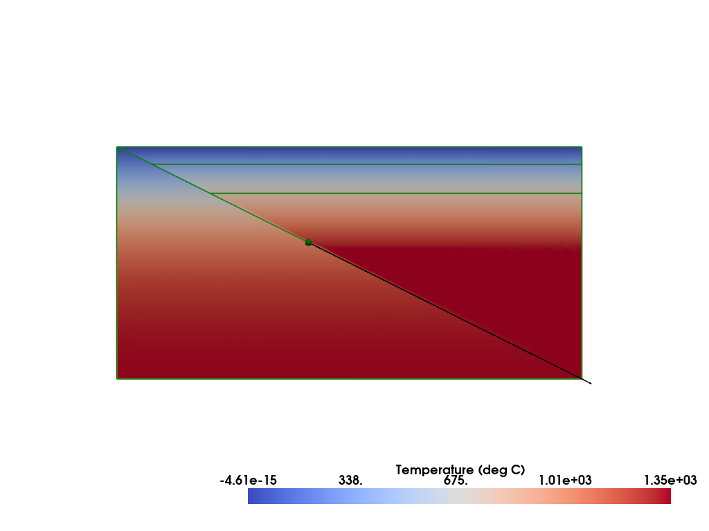
At this stage we expect to have generated the mesh, set up the function spaces and functions and initialized the initial conditions to their correct values. We can check this by plotting the current solution functions.
plotter_ic = fenics_sz.utils.plot.plot_scalar(sz_case1.T_i, scale=sz_case1.T0, gather=True, cmap='coolwarm', scalar_bar_args={'title': 'Temperature (deg C)', 'bold':True})
fenics_sz.utils.plot.plot_vector_glyphs(sz_case1.vw_i, plotter=plotter_ic, gather=True, factor=0.1, color='k', scale=fenics_sz.utils.mps_to_mmpyr(sz_case1.v0))
sz_case1.geom.pyvistaplot(plotter=plotter_ic, color='green', width=2)
cdpt = sz_case1.geom.slab_spline.findpoint('Slab::FullCouplingDepth')
fenics_sz.utils.plot.plot_points([[cdpt.x, cdpt.y, 0.0]], plotter=plotter_ic, render_points_as_spheres=True, point_size=10.0, color='green')
fenics_sz.utils.plot.plot_show(plotter_ic)
fenics_sz.utils.plot.plot_save(plotter_ic, output_folder / "sz_problem_case1_ics.png")
Of course we still haven’t described our equations let alone solved anything yet. We will begin implementing our solution strategy in the next notebook