Steady-State Subduction Zone Setup

Contents

Steady-State Subduction Zone Setup#

Authors: Kidus Teshome, Cian Wilson

Themes and variations - global suite geometries#

In this notebook we will try using more realistic geometries from the global suite.

Preamble#

Let’s start by adding the path to the modules in the python folder to the system path (so we can find the our custom modules).

import sys, os
basedir = ''
if "__file__" in globals(): basedir = os.path.dirname(__file__)
sys.path.append(os.path.join(basedir, os.path.pardir, os.path.pardir, 'python'))

Then load everything we need from sz_problems and other modules.

import utils
from sz_problems.sz_params import default_params, allsz_params
from sz_problems.sz_slab import create_slab
from sz_problems.sz_geometry import create_sz_geometry
from sz_problems.sz_steady_isoviscous import SteadyIsoSubductionProblem
from sz_problems.sz_steady_dislcreep import SteadyDislSubductionProblem
import pathlib
output_folder = pathlib.Path(os.path.join(basedir, "output"))
output_folder.mkdir(exist_ok=True, parents=True)

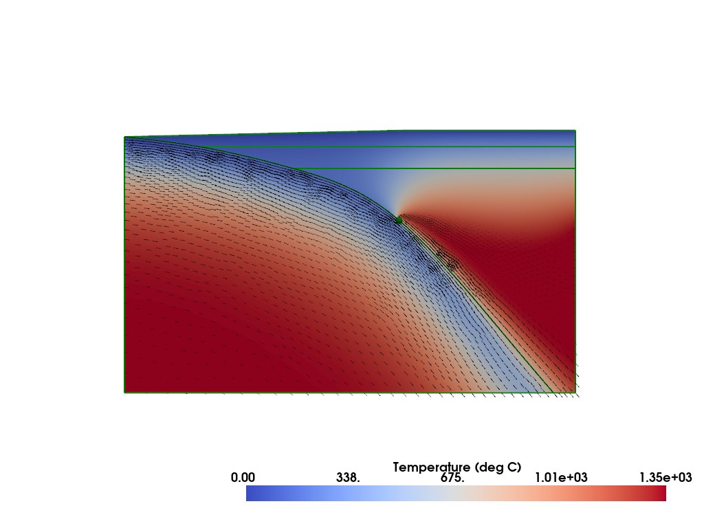
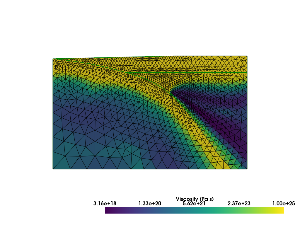
Alaska Peninsula (dislocation creep, low res)#

resscale_ak = 5.0
szdict_ak = allsz_params['01_Alaska_Peninsula']
slab_ak = create_slab(szdict_ak['xs'], szdict_ak['ys'], resscale_ak, szdict_ak['lc_depth'])
geom_ak = create_sz_geometry(slab_ak, resscale_ak, szdict_ak['sztype'], szdict_ak['io_depth'], szdict_ak['extra_width'], 
                             szdict_ak['coast_distance'], szdict_ak['lc_depth'], szdict_ak['uc_depth'])
sz_ak = SteadyDislSubductionProblem(geom_ak, **szdict_ak)

print("\nSolving steady state flow with isoviscous rheology...")
sz_ak.solve()

Solving steady state flow with isoviscous rheology...

Iteration   Residual     Relative Residual
------------------------------------------
0           7125.26      1           
1           811.298      0.113862    
2           108.535      0.0152324   

         60.4568      0.00848486  
         26.631       0.00373754  
         10.465       0.00146871  
         4.44722      0.000624148 

         2.16681      0.000304102 
         1.1928       0.000167404 
         0.719893     0.000101034 
        0.467766     6.5649e-05  

        0.3237       4.54299e-05 
        0.236329     3.31677e-05 
        0.180352     2.53116e-05 
        0.142387     1.99834e-05 

        0.115173     1.6164e-05  
        0.0946823    1.32883e-05 
        0.0786273    1.1035e-05  
        0.06567      9.21651e-06 

        0.0549949    7.7183e-06  
        0.0460837    6.46764e-06 
        0.0385896    5.41588e-06 
        0.0322656    4.52834e-06 

plotter_ak = utils.plot.plot_scalar(sz_ak.T_i, scale=sz_ak.T0, gather=True, cmap='coolwarm', scalar_bar_args={'title': 'Temperature (deg C)', 'bold':True})
utils.plot.plot_vector_glyphs(sz_ak.vw_i, plotter=plotter_ak, gather=True, factor=0.1, color='k', scale=utils.mps_to_mmpyr(sz_ak.v0))
utils.plot.plot_vector_glyphs(sz_ak.vs_i, plotter=plotter_ak, gather=True, factor=0.1, color='k', scale=utils.mps_to_mmpyr(sz_ak.v0))
sz_ak.geom.pyvistaplot(plotter=plotter_ak, color='green', width=2)
cdpt = sz_ak.geom.slab_spline.findpoint('Slab::FullCouplingDepth')
utils.plot.plot_points([[cdpt.x, cdpt.y, 0.0]], plotter=plotter_ak, render_points_as_spheres=True, point_size=10.0, color='green')
utils.plot.plot_show(plotter_ak)
utils.plot.plot_save(plotter_ak, output_folder / "sz_steady_tests_ak_solution.png")

eta_ak = sz_ak.project_dislocationcreep_viscosity()
plotter_eta_ak = utils.plot.plot_scalar(eta_ak, scale=sz_ak.eta0, gather=True, log_scale=True, show_edges=True, scalar_bar_args={'title': 'Viscosity (Pa s)', 'bold':True})
sz_ak.geom.pyvistaplot(plotter=plotter_eta_ak, color='green', width=2)
cdpt = sz_ak.geom.slab_spline.findpoint('Slab::FullCouplingDepth')
utils.plot.plot_points([[cdpt.x, cdpt.y, 0.0]], plotter=plotter_eta_ak, render_points_as_spheres=True, point_size=10.0, color='green')
utils.plot.plot_show(plotter_eta_ak)
utils.plot.plot_save(plotter_eta_ak, output_folder / "sz_steady_tests_ak_eta.png")

# clean up
del plotter_eta_ak
del sz_ak
del geom_ak
del slab_ak

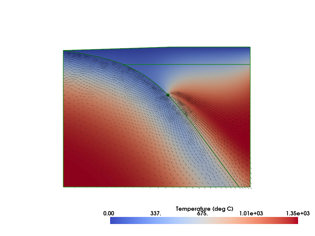
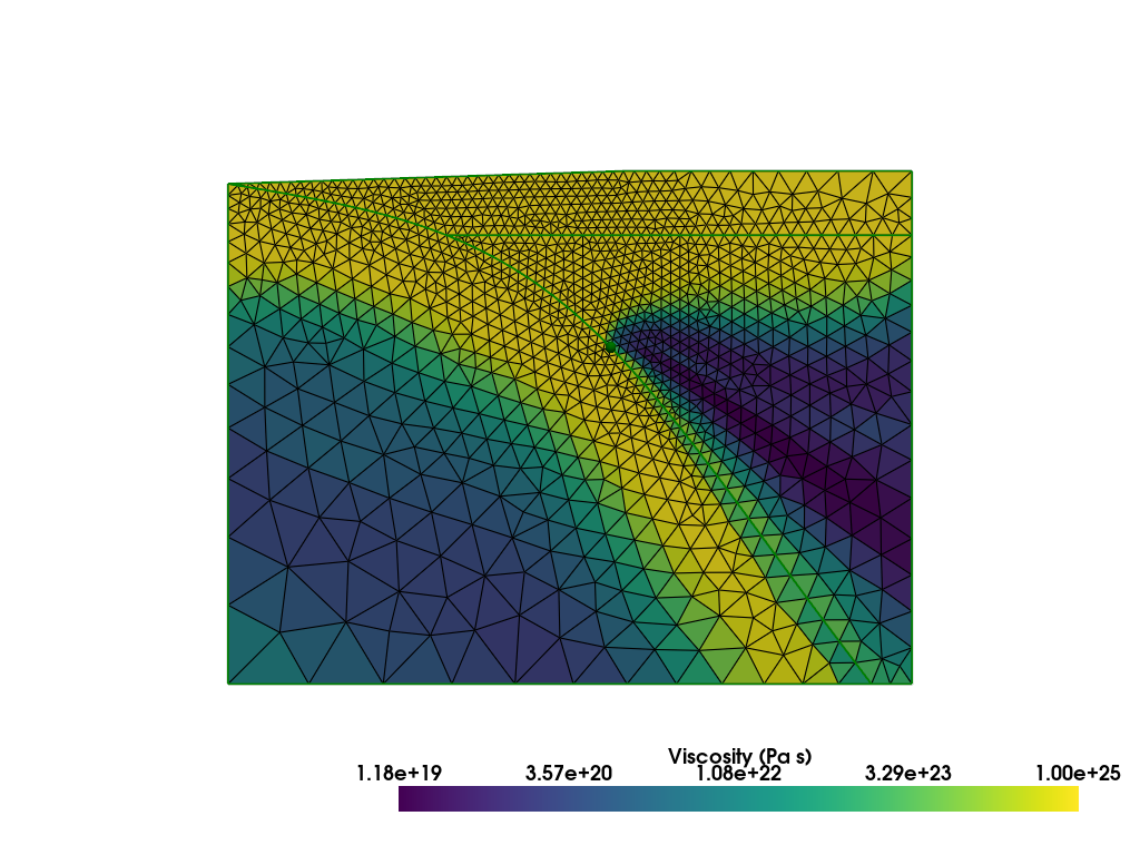
N Antilles (dislocation creep, low res)#

resscale_ant = 5.0
szdict_ant = allsz_params['19_N_Antilles']
slab_ant = create_slab(szdict_ant['xs'], szdict_ant['ys'], resscale_ant, szdict_ant['lc_depth'])
geom_ant = create_sz_geometry(slab_ant, resscale_ant, szdict_ant['sztype'], szdict_ant['io_depth'], szdict_ant['extra_width'], 
                              szdict_ant['coast_distance'], szdict_ant['lc_depth'], szdict_ant['uc_depth'])
sz_ant = SteadyDislSubductionProblem(geom_ant, **szdict_ant)

print("\nSolving steady state flow with isoviscous rheology...")
sz_ant.solve()

Solving steady state flow with isoviscous rheology...

Iteration   Residual     Relative Residual
------------------------------------------
0           4821.23      1           
1           2813.69      0.583604    
2           233.101      0.0483489   
3           88.591       0.0183752   

         38.3363      0.00795156  
         19.2591      0.00399464  
         10.9435      0.00226986  
         6.64963      0.00137924  
         4.35547      0.000903393 

         3.09337      0.000641614 
        2.33995      0.000485342 
        1.83278      0.000380147 
        1.45825      0.000302465 

        1.16782      0.000242225 
        0.940906     0.000195159 
        0.757093     0.000157033 
        0.604835     0.000125452 
        0.479977     9.95548e-05 

        0.379908     7.87989e-05 
        0.299543     6.213e-05   
        0.235121     4.87677e-05 
        0.183763     3.81154e-05 

        0.143067     2.96743e-05 
        0.110997     2.30225e-05 
        0.0858494    1.78065e-05 
        0.066217     1.37344e-05 
        0.0509492    1.05677e-05 

        0.0391163    8.11333e-06 
        0.0299733    6.21693e-06 
        0.0229277    4.75557e-06 

plotter_ant = utils.plot.plot_scalar(sz_ant.T_i, scale=sz_ant.T0, gather=True, cmap='coolwarm', scalar_bar_args={'title': 'Temperature (deg C)', 'bold':True})
utils.plot.plot_vector_glyphs(sz_ant.vw_i, plotter=plotter_ant, gather=True, factor=0.25, color='k', scale=utils.mps_to_mmpyr(sz_ant.v0))
utils.plot.plot_vector_glyphs(sz_ant.vs_i, plotter=plotter_ant, gather=True, factor=0.25, color='k', scale=utils.mps_to_mmpyr(sz_ant.v0))
sz_ant.geom.pyvistaplot(plotter=plotter_ant, color='green', width=2)
cdpt = sz_ant.geom.slab_spline.findpoint('Slab::FullCouplingDepth')
utils.plot.plot_points([[cdpt.x, cdpt.y, 0.0]], plotter=plotter_ant, render_points_as_spheres=True, point_size=10.0, color='green')
utils.plot.plot_show(plotter_ant)
utils.plot.plot_save(plotter_ant, output_folder / "sz_steady_tests_ant_solution.png")

eta_ant = sz_ant.project_dislocationcreep_viscosity()
plotter_eta_ant = utils.plot.plot_scalar(eta_ant, scale=sz_ant.eta0, gather=True, log_scale=True, show_edges=True, scalar_bar_args={'title': 'Viscosity (Pa s)', 'bold':True})
sz_ant.geom.pyvistaplot(plotter=plotter_eta_ant, color='green', width=2)
cdpt = sz_ant.geom.slab_spline.findpoint('Slab::FullCouplingDepth')
utils.plot.plot_points([[cdpt.x, cdpt.y, 0.0]], plotter=plotter_eta_ant, render_points_as_spheres=True, point_size=10.0, color='green')
utils.plot.plot_show(plotter_eta_ant)
utils.plot.plot_save(plotter_eta_ant, output_folder / "sz_steady_tests_ant_eta.png")

# clean up
del plotter_eta_ant
del sz_ant
del geom_ant
del slab_ant

Having played with some test examples using a steady state solver we will next formally examine the published benchmark solutions and test how our implementation performs.