Poisson Example 2D#
Description#
As a reminder, in this case we are seeking the approximate solution to
in a unit square, \(\Omega=[0,1]\times[0,1]\), imposing the boundary conditions
The analytical solution to this problem is \(T(x,y) = \exp\left(x+\tfrac{y}{2}\right)\).
Parallel Scaling#
In the previous notebook we tested that the error in our implementation of a Poisson problem in two-dimensions converged as the number of elements or the polynomial degree increased - a key feature of any numerical scheme. Another important property of a numerical implementation, particularly in greater than one-dimension, is that they can scale in parallel. So-called strong scaling means that, as more computer processors are used, the time the calculation takes, known as the simulation wall time, decreases. (The alternative, weak scaling means that the wall time ideally stays the same if the number of elements is increased proportionally to the number of processors.)
Here we perform strong scaling tests on our function solve_poisson_2d from notebooks/02_background/2.3b_poisson_2d.ipynb.
Preamble#
We start by loading all the modules and functions we will require, including test_plot_convergence from python/background/poisson_2d_tests.py, which was automatically created at the end of notebooks/02_background/2.3c_poisson_2d_tests.ipynb.
import sys, os
basedir = ''
if "__file__" in globals(): basedir = os.path.dirname(__file__)
path = os.path.join(basedir, os.path.pardir, os.path.pardir, 'python')
sys.path.insert(0, path)
import fenics_sz.utils.ipp
from fenics_sz.background.poisson_2d_tests import test_plot_convergence
import matplotlib.pyplot as pl
import matplotlib.ticker as ticker
import numpy as np
import pathlib
output_folder = pathlib.Path(os.path.join(basedir, "output"))
output_folder.mkdir(exist_ok=True, parents=True)
Implementation#
We perform the strong parallel scaling test using a utility function (profile_parallel from python/utils/ipp.py) that loops over a list of the number of processors calling our function for a given number of elements, ne, and polynomial order p. It runs our function solve_poisson_2d a specified number of times and evaluates and returns the time taken for each of a number of requested steps.
# the list of the number of processors we will use
nprocs_scale = [1, 2, 4]

# the number of elements in each direction (total elements = 2*ne*ne)
ne = 128

# the polynomial degree of our temperature field
p = 1

# perform the calculation a set number of times
number = 1

# We are interested in the time to create the mesh,
# declare the function spaces, assemble the problem and solve it.
# From our implementation in `solve_poisson_2d` it is also
# possible to request the time to declare the Dirichlet and
# Neumann boundary conditions and the forms.
steps = [
          'Mesh', 'Function spaces',
          'Assemble', 'Solve',
         ]

# declare a dictionary to store the times each step takes
maxtimes = {}
Direct#
To start with we test the scaling with the default solver options, which is a direct LU decomposition using the MUMPS library implementation. We add some extra petsc_options so we can monitor the timing of MUMPS and we additionally create a function to return information about the number of active and ghost degrees and freedom on each process.
petsc_options = {'ksp_type' : 'preonly', 'pc_type' : 'lu', 'pc_factor_mat_solver_type' : 'mumps', 'mat_mumps_icntl_4': 2}

def extra_parallel_diagnostics(T):
    diag = dict()
    diag['ndofs']   = T.function_space.dofmap.index_map.size_local
    diag['nghosts'] = T.function_space.dofmap.index_map.num_ghosts
    return diag

maxtimes_d, maxmumpstimes_d, extradiagout_d  = fenics_sz.utils.ipp.profile_parallel(nprocs_scale, steps, path,
                                                'fenics_sz.background.poisson_2d', 'solve_poisson_2d',
                                                ne, p, number=number, include_mumps_times=True,
                                                extra_diagnostics_func=extra_parallel_diagnostics,
                                                petsc_options=petsc_options,
                                                output_filename=output_folder / '2d_poisson_scaling_direct.png')

# save maxtimes for comparison later
maxtimes['Direct'] = maxtimes_d
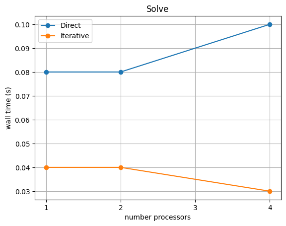
=========================
                     1           2           4
Mesh                 0.03        0.04        0.06
Function spaces      0           0           0
Assemble             0.01        0           0.01
Solve                0.08        0.08        0.1
=========================
MUMPS analysis       0.0552      0.0584      0.074
MUMPS factorization  0.019       0.0154      0.0163
MUMPS solve          0.002       0.0024      0.0026
=========================
ndofs_max            16641       8329        4190
ndofs_min            16641       8312        4128
ndofs_sum            16641       16641       16641
ndofs_avg            16641       8320.5      4160.25
nghosts_max          0           71          94
nghosts_min          0           58          63
nghosts_sum          0           129         291
nghosts_avg          0           64.5        72.75
=========================
*********** profiling figure in output/2d_poisson_scaling_direct.png
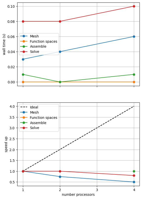
In the scaling test “speed up” is defined as the wall time on a given number of processors divided by the wall time on the smallest number of processors. Ideally this should increase linearly with the number of processors with slope 1. Such ideal scaling is rarely realized due to factors like the increasing costs of communication between processors but the behavior of the scaling test will also strongly depend on the computational resources available on the machine where this notebook is run. In particular when the website is generated it has to run as quickly as possible on github, hence we limit our requested numbers of processors, size of the problem (ne and p) and number of calculations to average over (number) in the default setup of this notebook.
For comparison we provide the output of this notebook using ne = 256, p = 2 and number = 10 in Figure 2.3.1 generated on a dedicated machine using a local conda installation of the software.
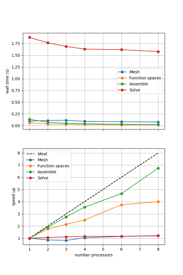
Figure 2.3.1 Scaling results for a direct solver with ne = 256, p = 2 averaged over number = 10 calculations using a local conda installation of the software on a dedicated machine.
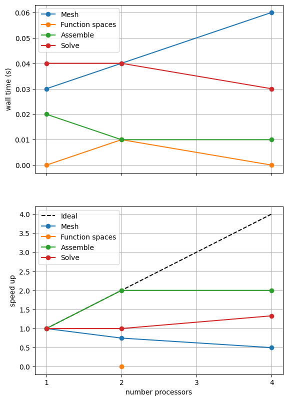
Here we can see that assembly and function space declarations scale well, with assembly being almost ideal. However meshing and the solve barely scale at all. The meshing takes place on a single process before being communicated to the other processors, hence we do not expect this step to scale. Additionally the cost (wall time taken) of meshing is so small that it is not a significant factor in these simulations. However the solution step is our most significant cost and would ideally scale. Its failure to do so here is a result of an initial analysis step that is performed by MUMPS in serial (on a single processor). We can see this by examining the timings in maxmumpstimes_d, which splits up the solve time into the analysis, factorization and solve steps of the MUMPS solver.
fig, (ax, ax_r) = pl.subplots(nrows=2, figsize=[6.4,9.6], sharex=True)
for k in maxmumpstimes_d[0].keys():
    ax.plot(nprocs_scale, [maxtimes[k] for maxtimes in maxmumpstimes_d], 'o-', label=k)
ax.xaxis.set_major_locator(ticker.MaxNLocator(integer=True))
ax.set_ylabel('wall time (s)')
ax.grid()
ax.legend()

ax_r.plot(nprocs_scale, [nproc/nprocs_scale[0] for nproc in nprocs_scale], 'k--', label='Ideal')
for k in maxmumpstimes_d[0].keys():
    ax_r.plot(nprocs_scale, maxmumpstimes_d[0][k]/np.asarray([maxtimes[k] for maxtimes in maxmumpstimes_d]), 'o-', label=k)
ax_r.xaxis.set_major_locator(ticker.MaxNLocator(integer=True))
ax_r.set_xlabel('number processors')
ax_r.set_ylabel('speed up')
ax_r.grid()
ax_r.legend()

fig.savefig(output_folder / '2d_poisson_scaling_direct_mumps.png')
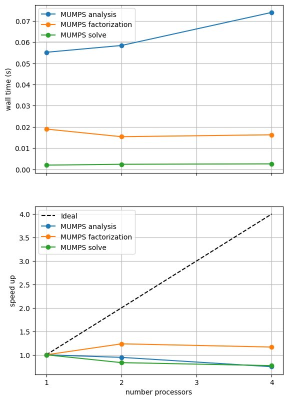
Again, behavior will depend on the machine this test is run on so we present a previously computed result using ne = 256, p = 2 and number = 10 in Figure 2.3.2 generated on a dedicated machine using a local conda installation of the software.
Figure 2.3.2 MUMPS scaling results for a direct solver with ne = 256, p = 2 averaged over number = 10 calculations using a local conda installation of the software on a dedicated machine.
Here we can see that the analysis step is what doesn’t scale at all (because by default it takes place in serial) while the factorization and solve steps take a lot less time and do scale (though not ideally). Because the analysis step is only performed once per matrix its cost will diminish relative to the other steps in nonlinear or time-dependent simulations where the matrix equation is solved multiple times.
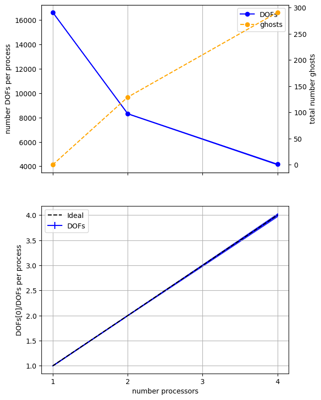
We can see why parallel simulations do not always scale perfectly by looking at the number of degrees of freedom on each process and the total number of ghost degrees of freedom.
fig, (ax, ax_r) = pl.subplots(nrows=2, figsize=[6.4,9.6], sharex=True)

ndofs_avg = np.asarray([extradiag['ndofs_avg'] for extradiag in extradiagout_d])
ndofs_min = np.asarray([extradiag['ndofs_min'] for extradiag in extradiagout_d])
ndofs_max = np.asarray([extradiag['ndofs_max'] for extradiag in extradiagout_d])
ndofs_errs = [np.abs(ndofs_min-ndofs_avg), np.abs(ndofs_max-ndofs_avg)]

lines = []
lines.append(ax.errorbar(nprocs_scale, ndofs_avg, yerr=ndofs_errs, c='blue', linestyle='-', marker='o', label='DOFs')[0])
lines[-1].set_label('DOFs')
ax.fill_between(nprocs_scale, ndofs_min, ndofs_max, color='blue')

nghosts_sum = np.asarray([extradiag['nghosts_sum'] for extradiag in extradiagout_d])

ax2 = ax.twinx()
lines.append(ax2.plot(nprocs_scale, nghosts_sum, c='orange', linestyle='--', marker='o', label='ghosts')[0])

ax.xaxis.set_major_locator(ticker.MaxNLocator(integer=True))
ax.set_ylabel('number DOFs per process')
ax2.set_ylabel('total number ghosts')
ax.grid(axis='x')
ax.legend(lines, [l.get_label() for l in lines])

ndofs_scale = ndofs_avg[0]/ndofs_avg
ndofs_scale_errs = [np.abs(ndofs_avg[0]/ndofs_max - ndofs_scale), np.abs(ndofs_avg[0]/ndofs_min - ndofs_scale)]

ax_r.plot(nprocs_scale, [nproc/nprocs_scale[0] for nproc in nprocs_scale], 'k--', label='Ideal', zorder=100)
ax_r.errorbar(nprocs_scale, ndofs_scale, yerr=ndofs_scale_errs, c='blue', linestyle='-', marker=None, label='DOFs')
ax_r.fill_between(nprocs_scale, ndofs_avg[0]/ndofs_max, ndofs_avg[0]/ndofs_min, color='blue', alpha=0.8)
ax_r.errorbar
ax_r.xaxis.set_major_locator(ticker.MaxNLocator(integer=True))
ax_r.set_xlabel('number processors')
ax_r.set_ylabel('DOFs[0]/DOFs per process')
ax_r.grid()
ax_r.legend()

fig.savefig(output_folder / '2d_poisson_scaling_direct_ndofs.png')
We present a previously computed result corresponding to the case with ne = 256, p = 2 and number = 10 in Figure 2.3.3 generated on a dedicated machine using a local conda installation of the software.
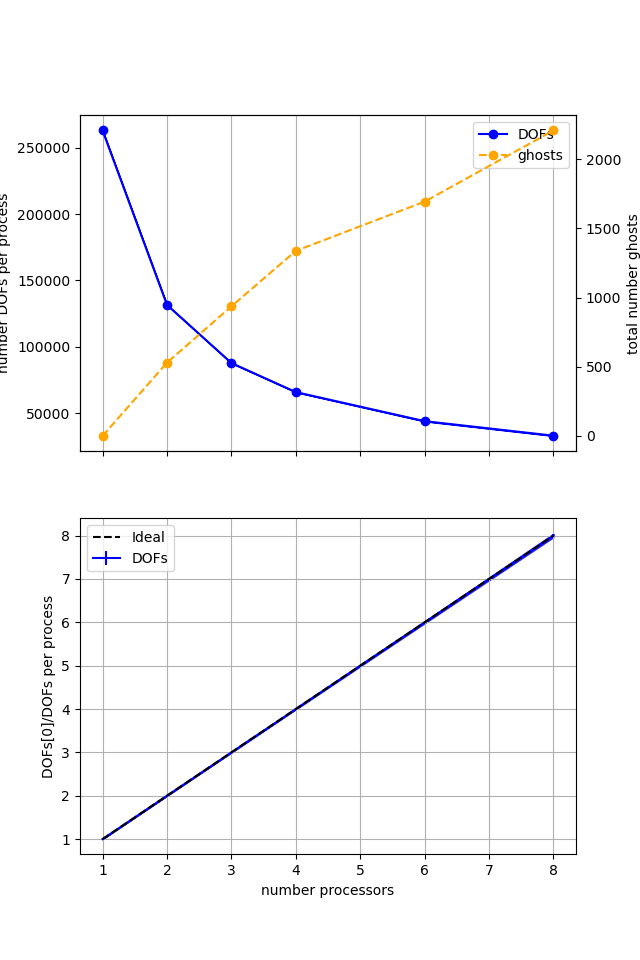
Figure 2.3.3 Numbers of degrees of freedom per process and the total number of ghost degrees of freedom with an increasing number of processes with ne = 256, p = 2 averaged over number = 10 calculations using a local conda installation of the software on a dedicated machine.
Here we can see that the number of degrees of freedom per process is decreasing (with the numbers of DOFs per process scaling ideally) with an increasing number of processes but the total (sum over all processes) of the ghost degrees of freedom is simultaneously increasing. So, while the cost per process is decreasing, the communications cost (as measured by the number of ghost degrees of freedom) is increasing, contributing to scaling not being ideal.
We will try different solution algorithms to get better behavior on a single solve but first we want to check that the solution is still converging in parallel. We do this by running our convergence test from notebooks/02_background/2.3c_poisson_tests.ipynb in parallel using another utility function utils.ipp.run_parallel.
# the list of the number of processors to test the convergence on
nprocs_conv = [2,]
# List of polynomial orders to try
ps = [1, 2]
# List of resolutions to try
nelements = [10, 20, 40, 80]
errors_l2_all = fenics_sz.utils.ipp.run_parallel(nprocs_conv, path, 'fenics_sz.background.poisson_2d_tests', 'convergence_errors', ps, nelements)

for errors_l2 in errors_l2_all:
    test_passes = test_plot_convergence(ps, nelements, errors_l2)
    assert(test_passes)
order of accuracy p=1, order=2.00
order of accuracy p=2, order=2.99

Iterative#
Having confirmed that our solution algorithm still converges in parallel we repeat the convergence test using an iterative solver (rather than a direct LU solver). We select a conjugate gradient (CG) iterative solver using a multi-grid (GAMG) preconditioner (with some additional tuning parameters) by passing the petsc_options dictionary to our function. We run over the same list of processors as before.
petsc_options = {'ksp_type' : 'cg', 'ksp_rtol' : 5.e-9, 'pc_type' : 'gamg', 'pc_gamg_threshold_scale' : 1.0, 'pc_gamg_threshold' : 0.01, 'pc_gamg_coarse_eq_limit' : 800}

maxtimes['Iterative'], _, _ = fenics_sz.utils.ipp.profile_parallel(nprocs_scale, steps, path,
                                                   'fenics_sz.background.poisson_2d', 'solve_poisson_2d',
                                                   ne, p, number=number, petsc_options=petsc_options,
                                                   output_filename=output_folder / '2d_poisson_scaling_iterative.png')
=========================
                 1           2           4
Mesh             0.03        0.04        0.06
Function spaces  0           0.01        0
Assemble         0.02        0.01        0.01
Solve            0.04        0.04        0.03
=========================
*********** profiling figure in output/2d_poisson_scaling_iterative.png
Again, results will depend on the computational resources available when the notebook is run and we intentionally limit the default parameters (nprocs_scale, ne, p and number) for website generation. We can compare against the output of this notebook using ne = 256, p = 2 and number = 10 in Figure 2.3.4 generated on a dedicated machine with a local conda installation of the software.
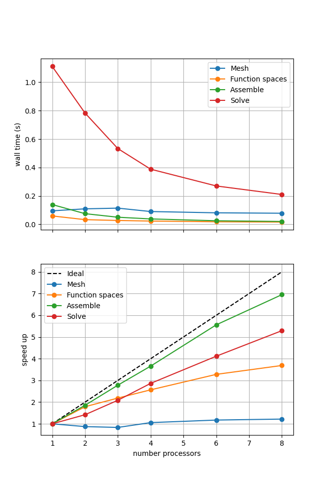
Figure 2.3.4 Scaling results for an iterative solver with ne = 256, p = 2 averaged over number = 10 calculations using a local conda installation of the software on a dedicated machine.
Here we can see that the solution algorithm scales much better than with the direct solver. We also need to check that the model is still converging by running our convergence test from notebooks/02_background/2.3c_poisson_tests.ipynb.
errors_l2_all = fenics_sz.utils.ipp.run_parallel(nprocs_conv, path, 'fenics_sz.background.poisson_2d_tests', 'convergence_errors', ps, nelements, petsc_options=petsc_options)

for errors_l2 in errors_l2_all:
    test_passes = test_plot_convergence(ps, nelements, errors_l2)
    assert(test_passes)
order of accuracy p=1, order=2.00
order of accuracy p=2, order=2.98
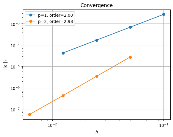
The iterative solver produces similar convergence results in parallel to the direct method. Note however that we had to set the iterative solver tolerance (ksp_rtol) to a smaller number than the default to achieve this at p = 2 and for small grid sizes (\(h\))/large numbers of elements (ne).
Comparison#
We can compare the wall time of the two solution algorithms directly.
# choose which steps to compare
compare_steps = ['Solve']

# set up a figure for plotting
fig, axs = pl.subplots(nrows=len(compare_steps), figsize=[6.4,4.8*len(compare_steps)], sharex=True)
if len(compare_steps) == 1: axs = [axs]
for i, step in enumerate(compare_steps):
    s = steps.index(step)
    for name, lmaxtimes in maxtimes.items():
        axs[i].plot(nprocs_scale, [t[s] for t in lmaxtimes], 'o-', label=name)
    axs[i].xaxis.set_major_locator(ticker.MaxNLocator(integer=True))
    axs[i].set_title(step)
    axs[i].legend()
    axs[i].set_ylabel('wall time (s)')
    axs[i].grid()
axs[-1].set_xlabel('number processors')
# save the figure
fig.savefig(output_folder / '2d_poisson_scaling_comparison.png')
Again, results will depend on the computational resources available when the notebook is run and we intentionally limit the default parameters (nprocs_scale, ne, p and number) for website generation. We can compare against the output of this notebook using ne = 256, p = 2 and number = 10 in Figure 2.3.5 generated on a dedicated machine with a local conda installation of the software.
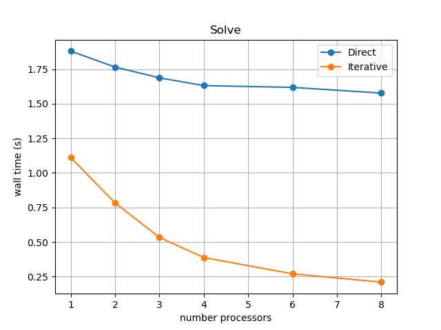
Figure 2.3.5 Scaling results for an iterative solver with ne = 256, p = 2 averaged over number = 10 calculations using a local conda installation of the software on a dedicated machine.
This emphasizes that not only does the iterative method continue to scale (decreasing wall time) to higher numbers of processors but its overall wall time is also lower than the direct method. We will see that this advantage decreases once more solves are performed in the simulation because the poor behavior of the direct method here is caused by a serial analysis step that, in our examples, only needs to be performed once per simulation.
Next we examine a more complicated case with two solution fields - a cornerflow problem where we are interested in finding both the velocity and pressure.