Blankenbach Thermal Convection Example#
Description#
As a reminder we are seeking the approximate velocity, pressure and temperature solutions of the coupled Stokes
and heat equations
in a bottom-heated unit square domain, \(\Omega\), with boundaries, \(\partial\Omega\).
For the Stokes problem we assume free-slip boundaries
and constrain the pressure to remove its null space, e.g. by applying a reference point
For the heat equation the side boundaries are insulating, the base hot and the top cold
We seek solutions at a variety of Rayleigh numbers, Ra, and consider both isoviscous, \(\eta = 1\), cases and a case with a temperature-dependent viscosity, \(\eta(T) = \exp(-bT)\) with \(b=\ln(10^3)\).
Parallel Scaling#
In the previous notebook we tested that the error in our implementation of a steady-state thermal convection problem in two-dimensions converged towards the published benchmark value as the number of elements increased. We also wish to test for parallel scaling of this problem, assessing if the simulation wall time decreases as the number of processors used to solve it increases.
Here we perform strong scaling tests on our function solve_blankenbach from notebooks/02_background/2.5b_blankenbach.ipynb. We will see that as we perform multiple solves in the Picard iteration the advantages of an iterative solver are eclipsed for this simple 2D case as the direct solver can reuse its initial expensive analysis step on subsequent solves. This also helps to overcome some of the poor scaling we observed using the direct solver in previous examples.
Preamble#
We start by loading all the modules we will require.
import sys, os
basedir = ''
if "__file__" in globals(): basedir = os.path.dirname(__file__)
path = os.path.join(basedir, os.path.pardir, os.path.pardir, 'python')
sys.path.insert(0, path)
import fenics_sz.utils.ipp
from fenics_sz.background.blankenbach import plot_convergence
import matplotlib.pyplot as pl
import matplotlib.ticker as ticker
import numpy as np
import pathlib
output_folder = pathlib.Path(os.path.join(basedir, "output"))
output_folder.mkdir(exist_ok=True, parents=True)
Implementation#
We perform the strong parallel scaling test using a utility function (profile_parallel from python/utils/ipp.py) that loops over a list of the number of processors calling our function for a given number of elements, ne, and pressure and temperature polynomial orders pp and pT. It runs our function solve_blankenbach a specified number of times and evaluates and returns the time taken for each of a number of requested steps.
# the list of the number of processors we will use
nprocs_scale = [1, 2, 4]

# the number of elements in each direction (total elements = 2*ne*ne)
ne = 128

# the polynomial degree of our pressure field
pp = 1
# the polynomial degree of our temperature field
pT = 1

# grid refinement factor
beta = 0.2

# perform the calculation a set number of times
number = 1

# We are interested in the time to create the mesh,
# declare the functions, assemble the problem and solve it.
# From our implementation in `solve_poisson_2d` it is also
# possible to request the time to declare the Dirichlet and
# Neumann boundary conditions and the forms.
steps = [
          'Assemble Temperature', 'Assemble Stokes',
          'Solve Temperature', 'Solve Stokes'
         ]
Case 1a - Direct#
We start by running case 1a - isoviscous with Ra \(=10^4\) - and will compare direct and iterative solver strategies.
# declare a dictionary to store the times each step takes
maxtimes_1a = {}
# case 1a
Ra = 1.e4
b = None # isoviscous
petsc_options_s = {'ksp_type':'preonly',
                   'pc_type':'lu',
                   'pc_factor_mat_solver_type' : 'mumps'
                  }

maxtimes_1a['Direct Stokes'], _, _ = fenics_sz.utils.ipp.profile_parallel(nprocs_scale, steps, path, 'fenics_sz.background.blankenbach', 'solve_blankenbach',
                                                        Ra, ne, pp=pp, pT=pT, b=b, beta=beta, number=number,
                                                        petsc_options_s=petsc_options_s,
                                                        output_filename=output_folder / 'blankenbach_scaling_direct_1a.png')
=========================
                      1           2           4
Assemble Temperature  0.19        0.12        0.11
Assemble Stokes       0.33        0.22        0.19
Solve Temperature     0.26        0.2         0.25
Solve Stokes          1.91        1.58        1.8
=========================
***********  profiling figure in output/blankenbach_scaling_direct_1a.png
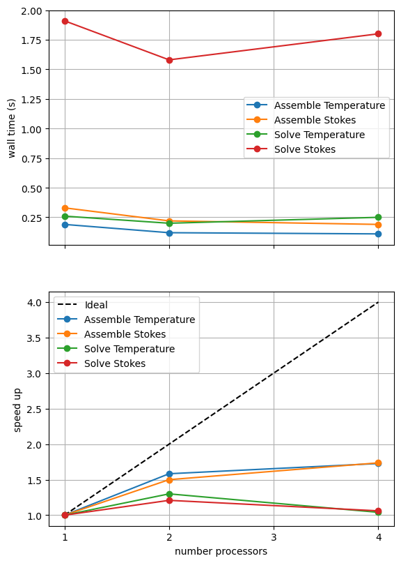
The behavior of the scaling test will strongly depend on the computational resources available on the machine where this notebook is run. In particular when the website is generated it has to run as quickly as possible on github, hence we limit our requested numbers of processors, size of the problem (ne, pp and pT) and number of calculations to average over (number) in the default setup of this notebook.
For comparison we provide the output of this notebook using ne = 256, pT = pp = 1, beta = 0.2 and number = 10 in Figure 2.5.1 generated on a dedicated machine with a local conda installation of the software.
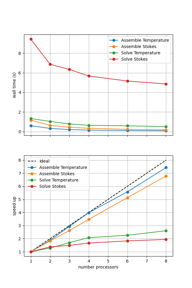
Figure 2.5.1 Scaling results for a direct solver with ne = 256, pT = pp = 1, beta = 0.2 averaged over number = 10 calculations using a local conda installation of the software on a dedicated machine.
We can see in Figure 2.5.1 that assembly scales well. Unlike in previous scaling tests we see that the solves also scale a little though far from ideally. This is because the expensive analysis step performed in serial (that prevented scaling on previous single solve cases) can be reused on subsequent solves within the Picard iteration of the Blankenbach problem, reducing the impact on the scaling and wall times.
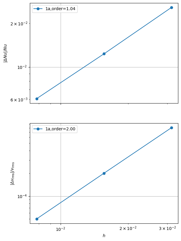
We also need to test that we are still converging to the benchmark solutions in parallel.
# the list of the number of processors to test the convergence on
nprocs_conv = [2,]

# List of polynomial orders to try
pTs = [1]
# List of resolutions to try
nelements = [32, 64, 128]
cases = ['1a']
errors_all = fenics_sz.utils.ipp.run_parallel(nprocs_conv, path, 'fenics_sz.background.blankenbach', 'convergence_errors', pTs, nelements, cases, beta=beta)

for errors in errors_all:
    fits = plot_convergence(pTs, nelements, errors)
    assert(all(fit > 1.0 for fits_p in fits.values() for fits_l in fits_p for fit in fits_l))
case 1a order of accuracy pT=1, Nu order=1.041330181998912, vrms order=2.00204608721493
Case 1a - Iterative#
In the previous cornerflow example the iterative solver overcame the scaling issues of the direct method so we once again test that strategy here.
# Case 1a
Ra = 1.e4
b=None
petsc_options_s = {'ksp_type':'minres',
                   'ksp_rtol': 5.e-8,
                   'pc_type':'fieldsplit',
                   'pc_fieldsplit_type': 'additive',
                   'fieldsplit_v_ksp_type':'preonly',
                   'fieldsplit_v_pc_type':'gamg',
                   'pc_gamg_threshold_scale' : 1.0,
                   'pc_gamg_threshold' : 0.01,
                   'pc_gamg_coarse_eq_limit' : 800,
                   'fieldsplit_p_ksp_type':'preonly',
                   'fieldsplit_p_pc_type':'jacobi'}

maxtimes_1a['Iterative (1a)'], _, _ = fenics_sz.utils.ipp.profile_parallel(nprocs_scale, steps, path, 'fenics_sz.background.blankenbach', 'solve_blankenbach',
                                                        Ra, ne, pp=pp, pT=pT, b=b, beta=beta,
                                                        petsc_options_s=petsc_options_s,
                                                        attach_nullspace=True,
                                                        number=number,
                                                        output_filename=output_folder / 'blankenbach_scaling_iterative_1a.png')
=========================
                      1           2           4
Assemble Temperature  0.19        0.1         0.1
Assemble Stokes       0.35        0.24        0.18
Solve Temperature     0.25        0.18        0.24
Solve Stokes          15.68       9.4         8.48
=========================
*********** profiling figure in output/blankenbach_scaling_iterative_1a.png
If sufficient computational resources are available when running this notebook (unlikely during website generation) this should show that the iterative method scales better than the direct method but has a much higher absolute cost (wall time).
For reference we provide the output of this notebook using ne = 256, pT = pp = 1, beta = 0.2 and number = 10 in Figure 2.5.2 generated on a dedicated machine with a local conda installation of the software.
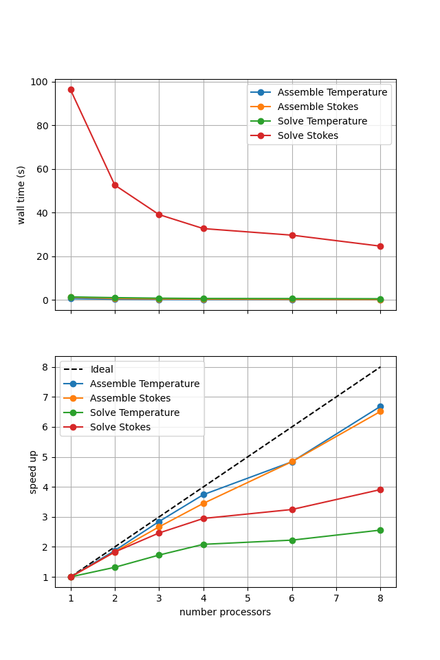
Figure 2.5.2 Scaling results for a direct solver with ne = 256, pT = pp = 1, beta = 0.2 averaged over number = 10 calculations using a local conda installation of the software on a dedicated machine.
Here we can see the improved scaling (for the Stokes solve, the temperature is still using a direct method) but increased cost. This is because each application of the iterative method selected here has roughly the same cost whereas the cost of the direct method reduces significantly on reapplication in later Picard iterations. Here we are performing roughly 10 iterations, which scales approximately with the relative costs of the two methods seen here.
We also test if the iterative method is converging to the benchmark solution below.
cases = ['1a']
errors_all = fenics_sz.utils.ipp.run_parallel(nprocs_conv, path,
                                    'fenics_sz.background.blankenbach', 'convergence_errors', pTs, nelements, cases, beta=beta,
                                    petsc_options_s=petsc_options_s,
                                    attach_nullspace=True)

for errors in errors_all:
    fits = plot_convergence(pTs, nelements, errors)
    assert(all(fit > 1.0 for fits_p in fits.values() for fits_l in fits_p for fit in fits_l))
case 1a order of accuracy pT=1, Nu order=1.041330330414761, vrms order=2.0020277340317696
Case 1a - Comparison#
We can more easily compare the different solution method directly by plotting their walltimes for assembly and solution.
# choose which steps to compare
compare_steps = ['Assemble Stokes', 'Solve Stokes']

# set up a figure for plotting
fig, axs = pl.subplots(nrows=len(compare_steps), figsize=[6.4,4.8*len(compare_steps)], sharex=True)
if len(compare_steps) == 1: axs = [axs]
for i, step in enumerate(compare_steps):
    s = steps.index(step)
    for name, lmaxtimes in maxtimes_1a.items():
        axs[i].plot(nprocs_scale, [t[s] for t in lmaxtimes], 'o-', label=name)
    axs[i].xaxis.set_major_locator(ticker.MaxNLocator(integer=True))
    axs[i].set_title(step)
    axs[i].legend()
    axs[i].set_ylabel('wall time (s)')
    axs[i].grid()
axs[-1].set_xlabel('number processors')
# save the figure
fig.savefig(output_folder / 'blankenbach_scaling_comparison_1a.png')
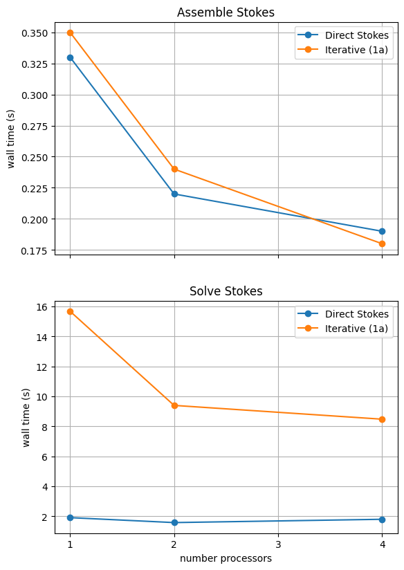
With sufficient computational resources we will see that both methods have approximately the same assembly costs but the iterative methods wall time costs are substantially higher and never become competitive despite scaling better at higher numbers of processors.
For reference we provide the output of this notebook using ne = 256, pT = pp = 1, beta = 0.2 and number = 10 in Figure 2.5.3 generated on a dedicated machine with a local conda installation of the software.
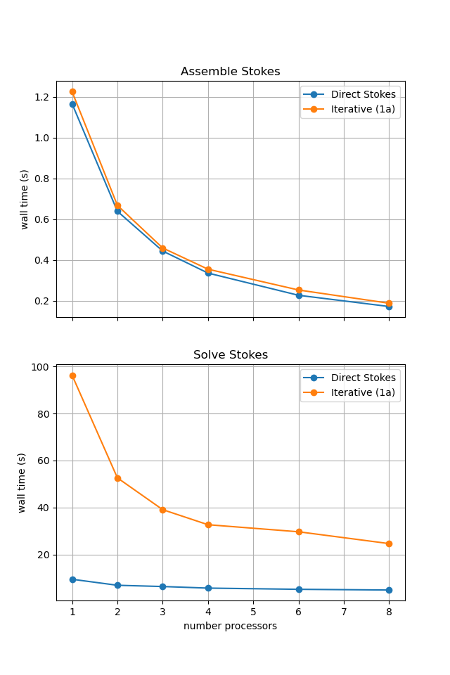
Figure 2.5.3 Scaling results for a direct solver with ne = 256, pT = pp = 1, beta = 0.2 averaged over number = 10 calculations using a local conda installation of the software on a dedicated machine.
Case 2a - Direct#
Time constraints mean we do not run case 2a (temperature-dependent rheology with Ra \(=10^4\)) but do present some previously run results below.
Uncommenting the cells below will allow the direct solution strategy to be tested interactively.
maxtimes_2a = {}
# # case 2a
# Ra = 1.e4
# b=np.log(1.e3) # temperature dependent viscosity
# petsc_options_s = {'ksp_type':'preonly',
#                    'pc_type':'lu',
#                    'pc_factor_mat_solver_type' : 'mumps'
#                   }

# maxtimes_2a['Direct Stokes'], _, _ = fenics_sz.utils.ipp.profile_parallel(nprocs_scale, steps, path, 'fenics_sz.background.blankenbach', 'solve_blankenbach',
#                                                         Ra, ne, pp=pp, pT=pT, b=b, beta=beta, number=number,
#                                                         petsc_options_s=petsc_options_s,
#                                                         output_filename=output_folder / 'blankenbach_scaling_direct_2a.png')
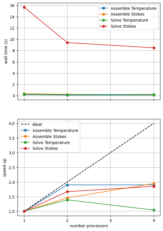
As before, if run interactively, the behavior of the scaling test will strongly depend on the computational resources available on the machine where this notebook is run.
For comparison we provide the output of this notebook using ne = 256, pT = pp = 1, beta = 0.2 and number = 10 in Figure 2.5.4 generated on a dedicated machine with a local conda installation of the software.
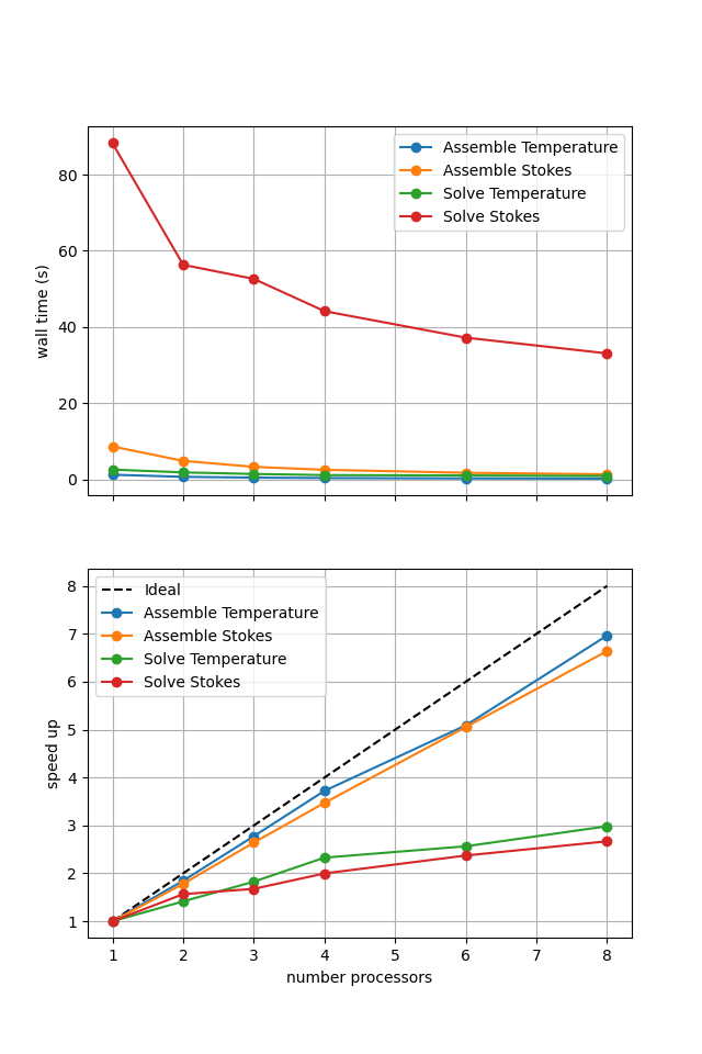
Figure 2.5.4 Scaling results for a direct solver with ne = 256, pT = pp = 1, beta = 0.2 averaged over number = 10 calculations using a local conda installation of the software on a dedicated machine.
We can see in Figure 2.5.4 that assembly scales well. The improved scaling behavior of the solves seen in case 1a is seen again and may even be marginally improved. This is likely because case 2a takes more iterations, further re-distributing the cost of the analysis step taken on the first iteration.
We can also test that we are still converging to the benchmark solutions in parallel by uncommenting the code below.
# cases = ['2a']
# errors_all = fenics_sz.utils.ipp.run_parallel(nprocs_conv, path, 'fenics_sz.background.blankenbach', 'convergence_errors', pTs, nelements, cases, beta=beta)

# for errors in errors_all:
#     fits = plot_convergence(pTs, nelements, errors)
#     assert(all(fit > 1.0 for fits_p in fits.values() for fits_l in fits_p for fit in fits_l))
Case 2a - Iterative#
Time constraints mean we do not run case 2a (temperature-dependent rheology with Ra \(=10^4\)) but do present some previously run results below.
Uncommenting the cells below will allow the iterative solution strategy to be tested interactively.
# # Case 2a
# Ra = 1.e4
# b=np.log(1.e3)
# petsc_options_s = {'ksp_type':'minres',
#                    'ksp_rtol': 5.e-9,
#                    'pc_type':'fieldsplit',
#                    'pc_fieldsplit_type': 'additive',
#                    'fieldsplit_v_ksp_type':'preonly',
#                    'fieldsplit_v_pc_type':'gamg',
#                    'pc_gamg_threshold_scale' : 1.0,
#                    'pc_gamg_threshold' : 0.01,
#                    'pc_gamg_coarse_eq_limit' : 800,
#                    'fieldsplit_p_ksp_type':'preonly',
#                    'fieldsplit_p_pc_type':'jacobi'}

# maxtimes_2a['Iterative Stokes'], _, _ = fenics_sz.utils.ipp.profile_parallel(nprocs_scale, steps, path, 'fenics_sz.background.blankenbach', 'solve_blankenbach',
#                                                         Ra, ne, pp=pp, pT=pT, b=b, beta=beta,
#                                                         petsc_options_s=petsc_options_s,
#                                                         attach_nullspace=True,
#                                                         number=number,
#                                                         output_filename=output_folder / 'blankenbach_scaling_iterative_2a.png')
If sufficient computational resources are available when running this cell interactively this should show that the iterative method scales better than the direct method but has a much higher absolute cost (wall time).
For reference we provide the output of this notebook using ne = 256, pT = pp = 1, beta = 0.2 and number = 10 in Figure 2.5.5 generated on a dedicated machine with a local conda installation of the software.
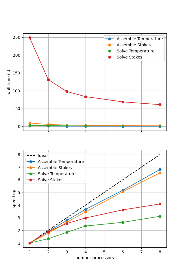
Figure 2.5.5 Scaling results for a direct solver with ne = 256, pT = pp = 1, beta = 0.2 averaged over number = 10 calculations using a local conda installation of the software on a dedicated machine.
Here we can see the improved scaling (for the Stokes solve, the temperature is still using a direct method) but hugely increased cost. This increase is even more significant here as the higher degree of non-linearity in case 2a compared to 1a has increased the number of nonlinear iterations taken.
We can also test if the iterative method is converging to the benchmark solution by uncommenting the cells below.
# cases = ['2a']
# errors_all = fenics_sz.utils.ipp.run_parallel(nprocs_conv, path,
#                                     'fenics_sz.background.blankenbach', 'convergence_errors', pTs, nelements, cases, beta=beta,
#                                     petsc_options_s=petsc_options_s,
#                                     attach_nullspace=True)

# for errors in errors_all:
#     fits = plot_convergence(pTs, nelements, errors)
#     assert(all(fit > 1.0 for fits_p in fits.values() for fits_l in fits_p for fit in fits_l))
Case 2a - Comparison#
Time constraints mean we do not run case 2a (temperature-dependent rheology with Ra \(=10^4\)) but do present some previously run results below.
Uncommenting the cells below will allow the solution strategies to be compared interactively.
# # choose which steps to compare
# compare_steps = ['Assemble Stokes', 'Solve Stokes']

# # set up a figure for plotting
# fig, axs = pl.subplots(nrows=len(compare_steps), figsize=[6.4,4.8*len(compare_steps)], sharex=True)
# if len(compare_steps) == 1: axs = [axs]
# for i, step in enumerate(compare_steps):
#     s = steps.index(step)
#     for name, lmaxtimes in maxtimes_2a.items():
#         axs[i].plot(nprocs_scale, [t[s] for t in lmaxtimes], 'o-', label=name)
#     axs[i].xaxis.set_major_locator(ticker.MaxNLocator(integer=True))
#     axs[i].set_title(step)
#     axs[i].legend()
#     axs[i].set_ylabel('wall time (s)')
#     axs[i].grid()
# axs[-1].set_xlabel('number processors')
# # save the figure
# fig.savefig(output_folder / 'blankenbach_scaling_comparison_2a.png')
If running interactively with sufficient computational resources we will see that both methods have approximately the same assembly costs but the iterative methods wall time costs are substantially higher and never become competitive despite scaling better at higher number of processors due to the improved scaling of reapplying the direct method.
For reference we provide the output of this notebook using ne = 256, pT = pp = 1, beta = 0.2 and number = 10 in Figure 2.5.6 generated on a dedicated machine using a local conda installation of the software.
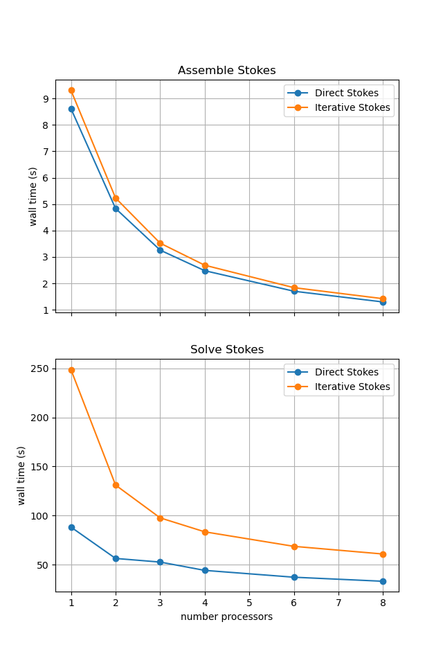
Figure 2.5.6 Scaling results for a direct solver with ne = 256, pT = pp = 1, beta = 0.2 averaged over number = 10 calculations using a local conda installation of the software on a dedicated machine.
In the next section we will apply what we have learned here to our implementation of a subduction zone thermal solver.