19 N Antilles

Authors: Kidus Teshome, Cian Wilson

Steady state implementation

Preamble

We are going to run this notebook in parallel using ipyparallel. To do this we launch a parallel engine with nprocs processes. Following this, all cells we wish to run in parallel need to start with the Jupyter magic %%px.

%%px

Cells without the %%px magic will run locally and will not have access to anything loaded on the parallel engine.

import ipyparallel as ipp
nprocs = 2
rc = ipp.Cluster(engine_launcher_class="mpi", n=nprocs).start_and_connect_sync()

Starting 2 engines with <class 'ipyparallel.cluster.launcher.MPIEngineSetLauncher'>

Set some path information.

%%px
import sys, os
basedir = ''
if "__file__" in globals(): basedir = os.path.dirname(__file__)
sys.path.append(os.path.join(basedir, os.path.pardir, os.path.pardir, os.path.pardir, 'python'))

Loading everything we need from sz_problem and also set our default plotting and output preferences.

%%px
import utils
from sz_problems.sz_params import allsz_params
from sz_problems.sz_slab import create_slab, plot_slab
from sz_problems.sz_geometry import create_sz_geometry
from sz_problems.sz_steady_dislcreep import SteadyDislSubductionProblem
import numpy as np
import dolfinx as df
import pyvista as pv
import pathlib
output_folder = pathlib.Path(os.path.join(basedir, "output"))
output_folder.mkdir(exist_ok=True, parents=True)
import hashlib
import zipfile
import requests
from mpi4py import MPI
comm = MPI.COMM_WORLD
my_rank = comm.rank

Parameters

We first select the name and resolution scale, resscale of the model.

Resolution

By default the resolution is low to allow for a quick runtime and smaller website size. If sufficient computational resources are available set a lower resscale to get higher resolutions and results with sufficient accuracy.

%%px
name = "19_N_Antilles"
resscale = 3.0

Then load the remaining parameters from the global suite.

%%px
szdict = allsz_params[name]
if my_rank == 0:
    print("{}:".format(name))
    print("{:<20} {:<10}".format('Key','Value'))
    print("-"*85)
    for k, v in allsz_params[name].items():
        if v is not None and k not in ['z0', 'z15']: print("{:<20} {}".format(k, v))

[stdout:0] 19_N_Antilles:
Key                  Value     
-------------------------------------------------------------------------------------
coast_distance       185
extra_width          19
lc_depth             30
io_depth             172
dirname              19_N_Antilles
As                   40.0
Ac                   90.0
A                    85
sztype               oceanic
Vs                   17.6
xs                   [0, 50.0, 102.2, 166.0, 176.5, 179.0, 195.0, 271.0, 301.0]
ys                   [-6, -15.0, -30.0, -70.0, -80.0, -82.5, -100.0, -200.0, -240.0]

Any of these can be modified in the dictionary.

Several additional parameters can be modified, for details see the documentation for the SteadyDislSubductionProblem class.

%%px
if my_rank == 0: help(SteadyDislSubductionProblem.__init__)

[stdout:0] Help on function __init__ in module sz_problems.sz_base:

__init__(self, geom, **kwargs)
    Initialize a BaseSubductionProblem.

    Arguments:
      * geom  - an instance of a subduction zone geometry

    Keyword Arguments:
     required:
      * A      - age of subducting slab (in Myr) [required]
      * Vs     - incoming slab speed (in mm/yr) [required]
      * sztype - type of subduction zone (either 'continental' or 'oceanic') [required]
      * Ac     - age of the over-riding plate (in Myr) [required if sztype is 'oceanic']
      * As     - age of subduction (in Myr) [required if sztype is 'oceanic']
      * qs     - surface heat flux (in W/m^2) [required if sztype is 'continental']

     optional:
      * Ts   - surface temperature (deg C, corresponds to non-dim)
      * Tm   - mantle temperature (deg C, corresponds to non-dim)
      * kc   - crustal thermal conductivity (non-dim) [only has an effect if sztype is 'continental']
      * km   - mantle thermal conductivity (non-dim)
      * rhoc - crustal density (non-dim) [only has an effect if sztype is 'continental']
      * rhom - mantle density (non-dim)
      * cp   - isobaric heat capacity (non-dim)
      * H1   - upper crustal volumetric heat production (non-dim) [only has an effect if sztype is 'continental']
      * H2   - lower crustal volumetric heat production (non-dim) [only has an effect if sztype is 'continental']

     optional (dislocation creep rheology):
      * etamax - maximum viscosity (Pas) [only relevant for dislocation creep rheologies]
      * nsigma - stress viscosity power law exponents (non-dim) [only relevant for dislocation creep rheologies]
      * Aeta   - pre-exponential viscosity constant (Pa s^(1/n)) [only relevant for dislocation creep rheologies]
      * E      - viscosity activation energy (J/mol) [only relevant for dislocation creep rheologies]

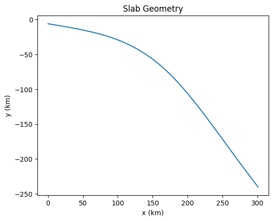
Setup

Setup a slab.

%%px
slab = create_slab(szdict['xs'], szdict['ys'], resscale, szdict['lc_depth'])
if my_rank == 0: _ = plot_slab(slab)

[output:0]

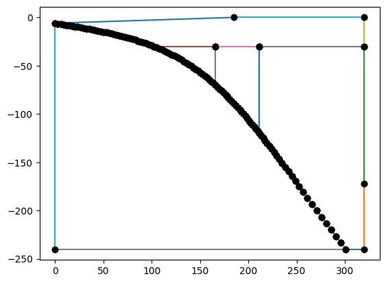
Create the subduction zome geometry around the slab.

%%px
geom = create_sz_geometry(slab, resscale, szdict['sztype'], szdict['io_depth'], szdict['extra_width'], 
                             szdict['coast_distance'], szdict['lc_depth'], szdict['uc_depth'])
if my_rank == 0: _ = geom.plot()

[output:0]

Finally, declare the SubductionZone problem class using the dictionary of parameters.

%%px
sz = SteadyDislSubductionProblem(geom, **szdict)

Solve

Solve using a dislocation creep rheology and assuming a steady state.

%%px
sz.solve()

[stdout:0] Iteration   Residual     Relative Residual
------------------------------------------
0           3766.54      1           
1           2372.66      0.629931    
2           225.708      0.0599244   
3           74.1707      0.019692    
4           38.5873      0.0102448   
5           22.1516      0.00588116  
6           13.8442      0.00367558  
7           9.27558      0.00246263  
8           6.58427      0.00174809  
9           4.88305      0.00129643  
10          3.73334      0.000991185 
11          2.90727      0.000771866 
12          2.28459      0.00060655  
13          1.80141      0.000478266 
14          1.42081      0.000377218 
15          1.11831      0.000296907 
16          0.876989     0.000232837 
17          0.68495      0.000181851 
18          0.532777     0.00014145  
19          0.412794     0.000109595 
20          0.318672     8.4606e-05  
21          0.24497      6.50385e-05 
22          0.187653     4.98212e-05 
23          0.143288     3.80424e-05 
24          0.109087     2.89621e-05 
25          0.0828203    2.19884e-05 
26          0.0627198    1.66518e-05 
27          0.0473891    1.25816e-05 
28          0.0357323    9.48677e-06 
29          0.0268939    7.14022e-06 
30          0.0202097    5.36559e-06 
31          0.0151662    4.02655e-06 

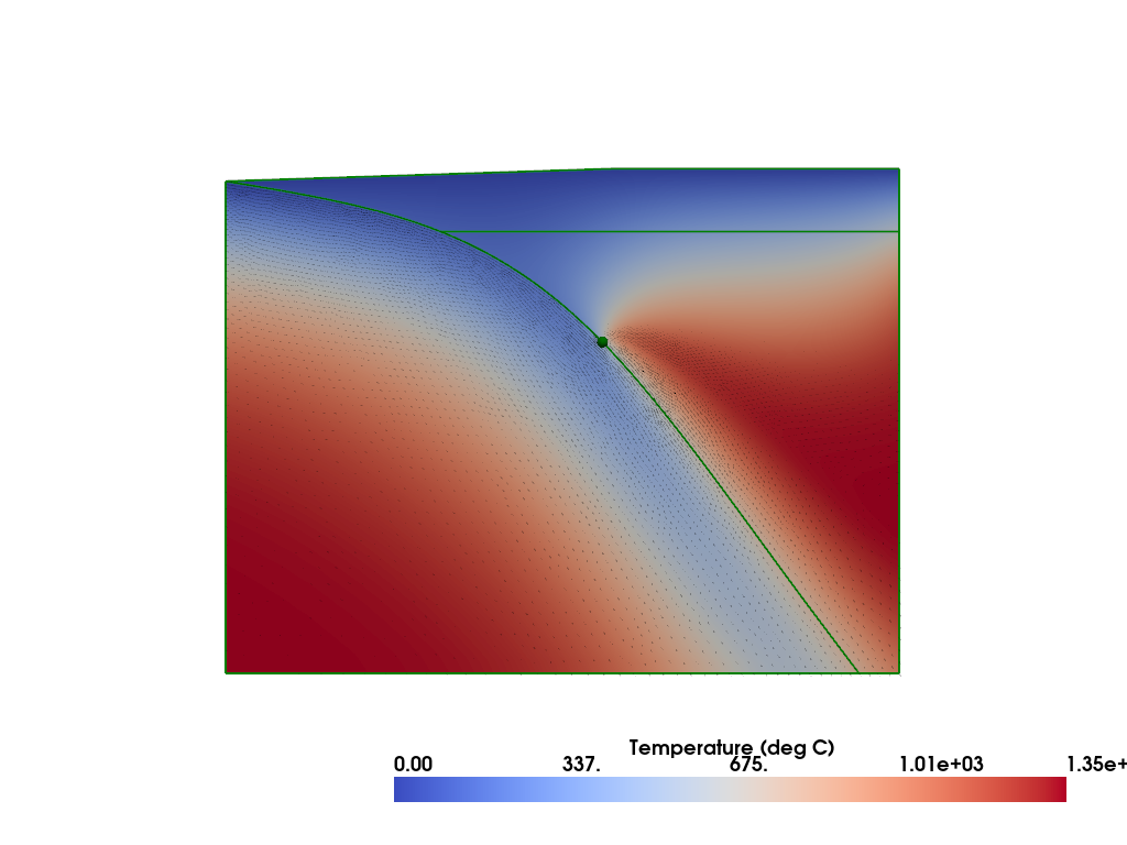
Plot

Plot the solution.

%%px
plotter = pv.Plotter()
utils.plot.plot_scalar(sz.T_i, plotter=plotter, scale=sz.T0, gather=True, cmap='coolwarm', scalar_bar_args={'title': 'Temperature (deg C)', 'bold':True})
utils.plot.plot_vector_glyphs(sz.vw_i, plotter=plotter, gather=True, factor=0.1, color='k', scale=utils.mps_to_mmpyr(sz.v0))
utils.plot.plot_vector_glyphs(sz.vs_i, plotter=plotter, gather=True, factor=0.1, color='k', scale=utils.mps_to_mmpyr(sz.v0))
geom.pyvistaplot(plotter=plotter, color='green', width=2)
cdpt = slab.findpoint('Slab::FullCouplingDepth')
utils.plot.plot_points([[cdpt.x, cdpt.y, 0.0]], plotter=plotter, render_points_as_spheres=True, point_size=10.0, color='green')
if my_rank == 0: 
    utils.plot.plot_show(plotter)
    utils.plot.plot_save(plotter, output_folder / "{}_ss_solution_resscale_{:.2f}.png".format(name, resscale))

[output:0]

Save it to disk so that it can be examined with other visualization software (e.g. Paraview).

%%px
filename = output_folder / "{}_ss_solution_resscale_{:.2f}.bp".format(name, resscale)
with df.io.VTXWriter(sz.mesh.comm, filename, [sz.T_i, sz.vs_i, sz.vw_i]) as vtx:
    vtx.write(0.0)
# zip the .bp folder so that it can be downloaded from jupyter lab
zipfilename = filename.with_suffix(".zip")
!zip -r $zipfilename $filename

[stdout:1]   adding: output/19_N_Antilles_ss_solution_resscale_3.00.bp/ (stored 0%)
  adding: output/19_N_Antilles_ss_solution_resscale_3.00.bp/data.0 (deflated 63%)
  adding: output/19_N_Antilles_ss_solution_resscale_3.00.bp/md.idx (deflated 59%)
  adding: output/19_N_Antilles_ss_solution_resscale_3.00.bp/mmd.0 (deflated 64%)
  adding: output/19_N_Antilles_ss_solution_resscale_3.00.bp/md.0 (deflated 85%)
  adding: output/19_N_Antilles_ss_solution_resscale_3.00.bp/profiling.json (deflated 72%)

[stdout:0]   adding: output/19_N_Antilles_ss_solution_resscale_3.00.bp/ (stored 0%)
  adding: output/19_N_Antilles_ss_solution_resscale_3.00.bp/data.0 (deflated 63%)
  adding: output/19_N_Antilles_ss_solution_resscale_3.00.bp/md.idx (deflated 59%)
  adding: output/19_N_Antilles_ss_solution_resscale_3.00.bp/mmd.0 (deflated 64%)
  adding: output/19_N_Antilles_ss_solution_resscale_3.00.bp/md.0 (deflated 85%)
  adding: output/19_N_Antilles_ss_solution_resscale_3.00.bp/profiling.json (deflated 72%)

Comparison

Compare to the published result from Wilson & van Keken, PEPS, 2023 (II) and van Keken & Wilson, PEPS, 2023 (III). The original models used in these papers are also available as open-source repositories on github and zenodo.

First download the minimal necessary data from zenodo and check it is the right version.

%%px
zipfilename = pathlib.Path(os.path.join(basedir, os.path.pardir, os.path.pardir, os.path.pardir, "data", "vankeken_wilson_peps_2023_TF_lowres_minimal.zip"))
# only one process should download the data
if my_rank == 0:
    if not zipfilename.is_file():
        zipfileurl = 'https://zenodo.org/records/13234021/files/vankeken_wilson_peps_2023_TF_lowres_minimal.zip'
        r = requests.get(zipfileurl, allow_redirects=True)
        open(zipfilename, 'wb').write(r.content)
# wait until rank 0 has downloaded the data
comm.barrier()
assert hashlib.md5(open(zipfilename, 'rb').read()).hexdigest() == 'a8eca6220f9bee091e41a680d502fe0d'

%%px
tffilename = os.path.join('vankeken_wilson_peps_2023_TF_lowres_minimal', 'sz_suite_ss', szdict['dirname']+'_minres_2.00.vtu')
tffilepath = os.path.join(basedir, os.path.pardir, os.path.pardir, os.path.pardir, 'data')
# one process should extract the file
if my_rank == 0:
    with zipfile.ZipFile(zipfilename, 'r') as z:
        z.extract(tffilename, path=tffilepath)
# other processes should wait
comm.barrier()

%%px
fxgrid = utils.plot.grids_scalar(sz.T_i)[0]

tfgrid = pv.get_reader(os.path.join(tffilepath, tffilename)).read()

diffgrid = utils.plot.pv_diff(fxgrid, tfgrid, field_name_map={'T':'Temperature::PotentialTemperature'}, pass_point_data=True)

%%px
# first gather the data onto rank 0
diffgrid_g = utils.plot.pyvista_grids(diffgrid.cells, diffgrid.celltypes, diffgrid.points, comm, gather=True)
T_g = comm.gather(diffgrid.point_data['T'], root=0)
for r, grid in enumerate(diffgrid_g):
    grid.point_data['T'] = T_g[r]
    grid.set_active_scalars('T')
    grid.clean(tolerance=1.e-2)
diffgrid_g

# then plot it
plotter_diff = pv.Plotter()
clim = None
for grid in diffgrid_g: 
    plotter_diff.add_mesh(grid, cmap='coolwarm', clim=clim, scalar_bar_args={'title': 'Temperature Difference (deg C)', 'bold':True})
geom.pyvistaplot(plotter=plotter_diff, color='green', width=2)
cdpt = slab.findpoint('Slab::FullCouplingDepth')
#utils.plot.plot_points([[cdpt.x, cdpt.y, 0.0]], plotter=plotter_diff, render_points_as_spheres=True, point_size=10.0, color='green')
plotter_diff.enable_parallel_projection()
plotter_diff.view_xy()
if my_rank == 0: plotter_diff.show()

[output:0]

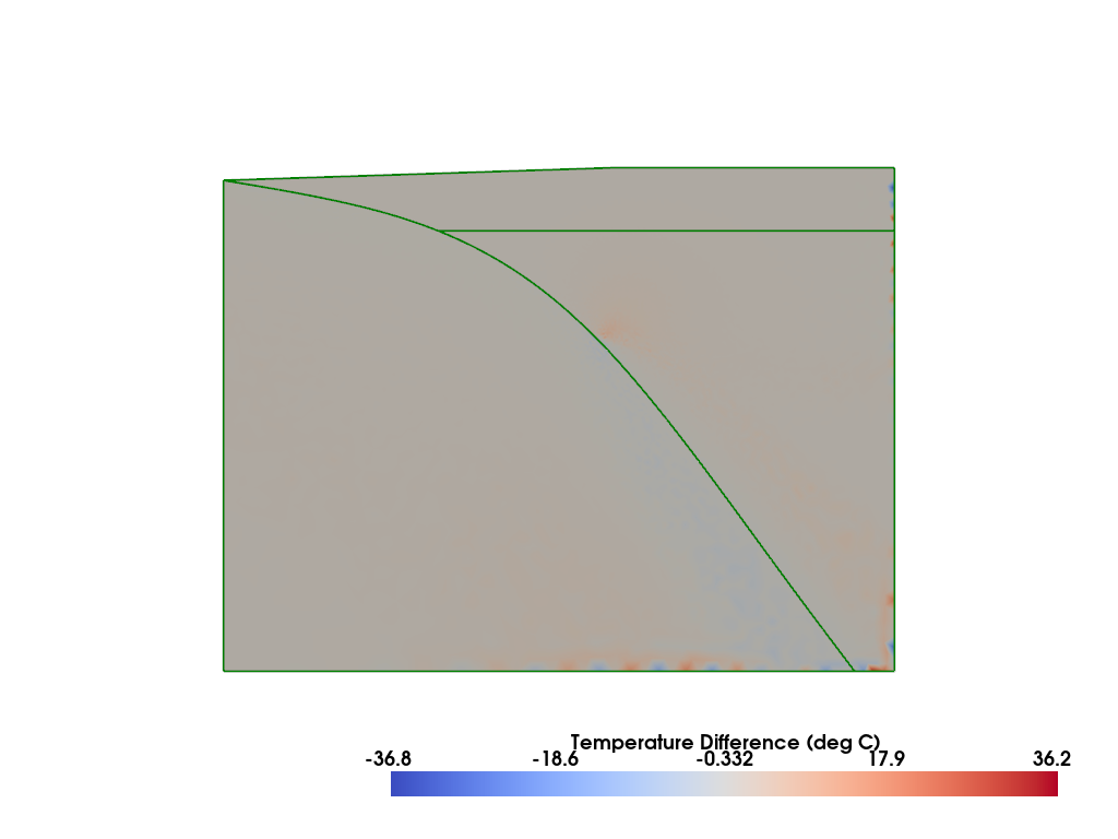
%%px
integrated_data = diffgrid.integrate_data()
totalarea = comm.allreduce(integrated_data['Area'][0], op=MPI.SUM)
error = comm.allreduce(integrated_data['T'][0], op=MPI.SUM)/totalarea
if my_rank == 0: print("Average error = {}".format(error,))
assert np.abs(error) < 5

[stdout:0] Average error = 0.3107185983164881