Subduction Zone Setup

Authors: Cian Wilson, Peter van Keken

Equations

We will start by formulating the full set of equations for subduction zone thermal structure. The equations will be introduced in dimensional form before nondimensionalizing them. All dimensional variables will be indicated by a superscript \(^*\). Dimensional reference values will be indicated by the subscript \(_0\). We assume a 2D Cartesian coordinate system with coordinates \(\vec{x}^*=(x^*_1,x^*_2)^T=(x^*,y^*)^T=(x^*,-z^*)^T\) where \(z^*\) is depth.

Conservation of mass under the assumption that the fluid is incompressible leads to

(62)\[\begin{equation} \nabla^* \cdot \vec{v}^*~=~0 \end{equation}\]

where, in two-dimensions, \(\vec{v}^*=(v^*_1,v^*_2)^T = (v^*_x,v^*_y)^T\) is the velocity vector. Assuming all flow is driven by a kinematic boundary condition, conservation of momentum leads to the dimensional Stokes equation without buoyancy forces

(63)\[\begin{equation} -\nabla^* \cdot {\boldsymbol\tau^*} +\nabla^* P^* ~=~ 0 \end{equation}\]

where \(P^*\) is the dynamic pressure and \(\boldsymbol \tau^*\) is the deviatoric stress tensor given by

(64)\[\begin{equation} {\boldsymbol\tau^*} ~=~2 \eta^* { \dot{\boldsymbol\epsilon}^*} \end{equation}\]

Here, \(\eta^*\) is dynamic viscosity and \(\dot{\boldsymbol\epsilon}^*\) is the deviatoric strain-rate tensor with components

(65)\[\begin{equation} \dot{\epsilon}^*_{ij}~=~ \frac{1}{2} \left[ \frac{\partial v^*_i}{\partial x^*_j} + \frac{\partial v^*_j}{\partial x^*_i} \right] \label{eq:strainratetensor} \end{equation}\]

The time-dependent dimensional heat equation is given by

(66)\[\begin{equation} \rho^* {c_p}_0 \left( \frac{\partial T^*}{\partial t^*} + \vec{v}^* \cdot \nabla^* T^* \right) ~=~ \nabla^* \cdot \left( k^* \nabla^* T^* \right) +H^* \end{equation}\]

while, in cases where a steady state is assumed (\(\frac{\partial T^*}{\partial t^*}\)=0) temperature is governed by

(67)\[\begin{equation} \rho^* {c_p}_0 \vec{v}^* \cdot \nabla^* T^* ~=~ \nabla^* \cdot \left( k^* \nabla^* T^* \right) +H^* \end{equation}\]

where \(\rho^*\) is density, \({c_p}_0\) is the heat capacity at constant pressure (assumed constant), \(T^*\) is temperature, \(k^*\) is thermal conductivity, and \(H^*\) is volumetric heat production.

Here we will assume that the viscosity \(\eta^*\) is either constant, \(\eta^* = \eta_0\), or is a function of temperature and strain rate following a simplified creep law for dislocation creep in dry olivine

(68)\[\begin{equation} \eta^*_\text{disl}~=~ A_\eta^* \exp \left( \frac{E^*}{nR^*(T^*+T^*_a)} \right) {{\dot{\epsilon}_{II}}}^{*\frac{1-n}{n}} \end{equation}\]

where \(A_\eta^*\) is a prefactor, \(E^*\) is the activation energy, \(R^*\) is the gas constant, \(n\) is a powerlaw index, \(T^*_a\) a linear approximation of an adiabatic temperature using a gradient of 0.3\(^\circ\)C/km with \(T^*_a\)=0 at the top of the model (which may not be at \(z^*\)=0 due to assumptions of ocean bathymetry as we will see later, and \(\dot{\epsilon}_{II}^*\) is the second invariant of the deviatoric strain-rate tensor (also known as the effective deviatoric strain rate)

(69)\[\begin{equation} \dot{\epsilon}_{II}^*~=~ \sqrt{\frac{1}{2} \dot{\boldsymbol\epsilon}^*:\dot{\boldsymbol\epsilon}^*} \end{equation}\]

Since the dynamical range of the viscosity is large over the temperature contrast across subduction zones it is common practice to cap the viscosity at some arbitrary maximum \(\eta^*_\text{max}\) so that in the variable viscosity case

(70)\[\begin{equation} \eta^*~=~ \left( \frac{1}{\eta^*_\text{disl}} ~+~ \frac{1}{\eta^*_\text{max}}\right)^{-1} \end{equation}\]

Nondimensionalization

It is attractive to nondimensionalize the equations such that most quantities are scaled to be close to \(1\). This provides simple scaling arguments to allow for understanding which terms in the equations are dominant, avoids computer algebra that mixes very large and very small numbers, and provides for the formation of a matrix-vector system where the condition number of the matrix is more optimal.

Quantity	Symbol	Nominal value	Nondimensional value
Reference temperature scale	\( T_0\)	1 K=1\(^\circ\)C	-
Surface temperature	\(T^*_s\)	273 K=0\(^\circ\)C	\(T_s\)=0
Mantle temperature	\(T^*_m\)	1623 K=1350\(^\circ\)C	\(T_m\)=1350
Surface heat flow note{c}	\(q^*_s\)	\(^\S\) W/m\(^2\)	\(q_s\)\(^\S\)
Reference density	\(\rho_0\)	3300 kg/m\(^3\)	-
Crustal density\(^\text{c}\)	\(\rho^*_c\)	2750 kg/m\(^3\)	\(\rho_c\)=0.833333
Mantle density	\(\rho^*_m\)	3300 kg/m\(^3\)	\(\rho_m\)=1
Reference thermal conductivity	\(k_0\)	3.1 W/(m K)	-
Crustal thermal conductivity\(^\text{c}\)	\(k^*_c\)	2.5 W/(m K)	\(k_c\)=0.8064516
Mantle thermal conductivity	\(k^*_m\)	3.1 W/(m K)	\(k_m\)=1
Volumetric heat production (upper crust)\(^\text{c}\)	\(H^*_1\)	1.3 \(\mu\)W/m\(^3\)	\(H_1\)=0.419354
Volumetric heat production (lower crust)\(^\text{c}\)	\(H_2^*\)	0.27 \(\mu\)W/m\(^3\)	\(H_2\)=0.087097
Age of overriding crust\(^\text{o}\)	\(A_c^*\)	\(^\S\) Myr	\(A_c\)\(^\S\)
Age of subduction\(^\text{t}\)	\(A_s^*\)	\(^\S\) Myr	\(A_s\)\(^\S\)
Age of subducting slab	\(A^*\)	\(^\S\) Myr	\(A\)\(^\S\)
Reference length scale	\(h_0\)	1 km	-
Depth of base of upper crust\(^\text{c}\)	\(z_1^*\)	15 km	\(z_1\)=15
Depth of base of lower crust (Moho)	\(z_2^*\)	\(^\S\) km	\(z_2\)\(^\S\)
Trench depth	\(z_\text{trench}^*\)	\(^\S\) km	\(z_\text{trench}\)\(^\S\)
Position of the coast line	\(x_\text{coast}^*\)	\(^\S\) km	\(x_\text{coast}\)\(^\S\)
Wedge inflow/outflow transition depth	\(z_\text{io}^*\)	\(^\S\) km	\(z_\text{io}\)\(^\S\)
Depth of domain	\(D^*\)	\(^\S\) km	\(D\)\(^\S\)
Width of domain	\(L^*\)	\(^\S\) km	\(L\)\(^\S\)
Depth of change from decoupling to coupling	\(d_c^*\)	80 km	\(d_c\)=80
Reference heat capacity	\({c_p}_0\)	1250 J/(kg K)	-
Reference thermal diffusivity	\(\kappa_0\)	0.7515\(\times\)10\(^{\textrm{-6}}\) m\(^2\)/s	-
Activation energy	\(E\)	540 kJ/mol	-
Powerlaw exponent	\(n\)	3.5	-
Pre-exponential constant	\(A^*_\eta\)	28968.6 Pa s\(^{1/n}\)	-
Reference viscosity scale	\(\eta_0\)	10\(^{\textrm{21}}\) Pa s	-
Viscosity cap	\(\eta^*_\text{max}\)	10\(^{\textrm{25}}\) Pa s	-
Gas constant	\(R^*\)	8.3145 J/(mol K)	-
Derived velocity scale	\({v}_0\)	23.716014 mm/yr	-
Convergence velocity	\(V_s^*\)	\(^\S\) mm/yr	\(V_s\)\(^\S\)

\(^\text{c}\)	ocean-continent subduction only
\(^\text{o}\)	ocean-ocean subduction only
\(^\text{t}\)	time-dependent simulations only
\(^\S\)	varies between models

Table 1: Nomenclature and reference values

Table 1 provides a list of dimensional reference values, dimensional parameters, and their nondimensional equivalents. For the nondimensionalization of the equations we use the diffusional time scaling with nondimensional time defined as \(t = t^* \kappa_0 / h_0^2\) where \(h_0\) is the reference length scale and \(\kappa_0\) is the reference thermal diffusivity. With \(\vec{x} = \vec{x}^*/h_0\) it follows \(\vec{v} = \vec{v}^* h_0 / \kappa_0\), \(\dot{\epsilon} = \dot{\epsilon}^* h_0^2 / \kappa_0\), and \(\nabla = \nabla^* h_0\). We further introduce \(T = (T^*-T^*_s)/T_0\), \(k = k^* / k_0\), \(\rho = \rho^* / \rho_0\), \(P = P^* h^2_0 / (\kappa_0 \eta_0)\), and \(H = H^* h_0^2 / ( \rho_0 {c_p}_0 T_0 \kappa_0 )\). Note that our choices of \(T_0\) and \(h_0\) in Table 1 cause the numerical values of dimensional position (in km) and temperature (in \(^\circ\)C) to have the same magnitude as the corresponding nondimensional quantities. Substitution of the nondimensional variables and constants leads to the following set of nondimensional equations for pressure and velocity

(71)\[\begin{equation} \nabla \cdot \vec{v} = 0 \end{equation}\]

(72)\[\begin{equation} -\nabla \cdot \left(2\eta \frac{\nabla \vec{v} + \nabla \vec{v}^T}{2} \right) + \nabla P = 0 \end{equation}\]

and either a time-dependent equation for temperature

(73)\[\begin{equation} \rho \left( \frac{\partial T}{\partial t} + \vec{v} \cdot \nabla T \right) = \nabla \cdot \left( k \nabla T \right) + H \end{equation}\]

or its equivalent when a steady-state solution is assumed

(74)\[\begin{equation} \rho \vec{v} \cdot \nabla T = \nabla \cdot \left( k \nabla T \right) + H \end{equation}\]

The viscosity \(\eta\) is either constant \(1\) or follows from the dislocation creep formulation as

(75)\[\begin{equation} \eta=\frac{\eta^*}{\eta_0} \end{equation}\]

Note that for simplicity as well as clarity we form the viscosity function in dimensional form and nondimensionalize the viscosity with the reference viscosity \(\eta_0\).

Geometry

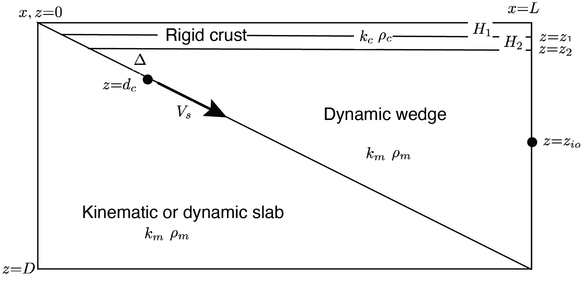Figure 1: Geometry and coefficients for a simplified 2D subduction zone model. All coefficients and parameters are nondimensional. The decoupling point is indicated by the star.

A simplified version of the typical geometry used in 2D subduction zone modeling with a kinematically prescribed slab is shown in Figure 1. The model is a 2D Cartesian box of width \(L\) and depth \(D\). We picture a model with a straight slab surface here but it can also be constructed from a natural spline through a set of control points as in Syracuse et al., PEPI, 2023 or connected linear segments with different angles with respect to the horizontal as in Wada & Wang, G3, 2009. In the global suite of models, which follow the geometries of Syracuse et al., PEPI, 2023, the simplified geometry in Figure 1 is modified by including a curved slab and a coastline. At \(x\)=0 the top of the model is at \((0,z_\text{trench})^T\), for a given depth of the trench, \(z_\text{trench}\). Between \(x\)=0 and \(x = x_\text{coast}\), the presumed horizontal position of the coast, the top of the model shallows linearly to \((x_\text{coast},0)^T\). For \(x>x_\text{coast}\) the top of the model is at \(z\)=0. Actual choices for these parameters are provided in the global suite.

The kinematic slab approach requires at a minimum that the slab surface velocity with magnitude \(V_s\) is prescribed. The velocity in the slab, \(\vec{v}_s\), can be determined from the solution of the Stokes (mass and momentum) equations in the slab. This requires us to solve these equations twice, once in the slab and once in the wedge owing to the discontinuity in velocity and pressure required across the slab above the coupling depth. Hence we solve the heat equation for temperature \(T\) in the whole domain and the Stokes equations twice, once in the wedge for \(\vec{v} = \vec{v}_w\) and \(P = P_w\) and once in the slab for \(\vec{v} = \vec{v}_s\) and \(P = P_s\). The velocity in the overriding plate, above the slab and down to \(z = z_2\), is always prescribed as \(\vec{v} = 0\) and the Stokes equations are not solved here.

Discretization

We use an unstructured mesh of triangular elements to discretize the domain. On this mesh we define discrete approximate discrete solutions for wedge velocity, wedge pressure, slab velocity, slab pressure, and temperature as

(76)\[\begin{align} \vec{v}_w \approx \tilde{\vec{v}}_w &= \sum_j\omega^k_j v^k_{wj} \\ P_w \approx \tilde{P}_w &= \sum_j \chi_j P_{wj} \\ \vec{v}_s \approx \tilde{\vec{v}}_s &= \sum_j \omega^k_j v^k_{sj} \\ P_s \approx \tilde{P}_s &= \sum_j \chi_j P_{sj} \\ T \approx \tilde{T} &= \sum_j \phi_j T_j \end{align}\]

with similarly defined discrete test functions, \(\tilde{\vec{v}}_{wt}\), \(\tilde{P}_{wt}\), \(\tilde{\vec{v}}_{st}\), \(\tilde{P}_{st}\), and \(\tilde{T}_t\) using the same shape functions \(\vec{\omega}_j = \omega^k_j\), \(\chi_j\) and \(\phi_j\) for velocity, pressure and temperature at each DOF \(j\) respectively. Here we use a P2P1P2 discretization where \(\vec{\omega}_j\) are piecewise-quadratic, \(\chi_j\) are piecewise-linear and \(\phi_j\) are piecewise-quadratic continuous Lagrange functions.

Boundary conditions

For the heat equation we assume homogeneous Neumann boundary conditions along the geometry where the velocity vector points out of the box (i.e., an outflow boundary). At the trench inflow boundary we assume a half-space cooling model \(T_\text{trench}(z)\) given by

(77)\[\begin{equation} \tilde{T}(x=0,z) = T_\text{trench}(z) = T_s + (T_m - T_s ) {\rm erf} \left( \tfrac{z-z_\text{trench}}{z_d} \right) \end{equation}\]

where \(T_s\) is the nondimensional surface temperature, \(T_m\) the nondimensional mantle temperature, \(z_\text{trench}\) is the nondimensional depth of the trench, and the nondimensional scale depth \(z_d\) is proportional to the dimensional age of the incoming lithosphere \(A^*\) via \(z_d = 2 \tfrac{\sqrt{ \kappa_0 A^*}}{h_0}\).

Details of the backarc temperature depend on whether we are modeling ocean-continent or ocean-ocean subduction. In the ocean-continent case we assume a constant surface heat flow \(q_s\) and radiogenic heat production \(H\). We use a two-layer crustal model with density \(\rho = \rho_c\), thermal conductivity \(k = k_c\) and heat production \(H = H_1\) from depth 0 to \(z_1\) and heat production \(H = H_2\) between depths \(z_1\) and \(z_2\), where \(z_1\) and \(z_2\) vary between subduction zones. The mantle portion of the model (in both the slab and the wedge) is assumed to have density \(\rho = \rho_m\), conductivity \(k = k_m\), and zero heat production \(H\)=0. At the backarc the wedge inflow boundary condition on temperature is chosen to be a geotherm \(T_\text{backarc}(z)\) consistent with these parameters, that is

(78)\[\begin{equation} \tilde{T}(x=L,z) = T_\text{backarc,c}(z) ~=~ \left\{ \begin{array}{l@{\quad:\quad}l} T_s -\frac{H_1 z^2}{2 k_c}~+~\frac{q_s}{k_c}z & 0 \leq z \leq z_1 \\ T_\text{backarc,c}(z=z_1)-\frac{H_2 (z-z_1)^2}{2 k_c} ~+~\frac{q_1}{k_c}(z-z_1) & z_1 < z \leq z_2 \\ \min(T_m,T_\text{backarc,c}(z=z_2)+\frac{q_2}{k_m}(z-z_2))& z_2 < z \leq z_\text{io} \end{array} \right. \end{equation}\]

The discrete heat flow values \(q_i\) are the heat flow at the crustal boundaries at depth \(z = z_i\) that can be found as \(q_1 = q_s - H_1 z_1\) and \(q_2 = q_1 - H_2 (z_2 - z_1)\). In the ocean-ocean case we use a one-layer crustal model (\(z_1\) is not defined), heat production is zero (\(H\)=0) and the density and thermal conductivity are set to respectively \(\rho = \rho_m\) and \(k = k_m\) everywhere. The wedge inflow boundary condition on temperature down to \(z_\text{io}\) is then

(79)\[\begin{equation} \tilde{T}(x=L,z) = T_\text{backarc,o}(z) ~=~ T_s + (T_m - T_s ) {\rm erf} \left( \tfrac{z}{z_c} \right) \end{equation}\]

where \(z_c\) is related to the dimensional age of the overriding plate \(A_c^*\) minus the age of subduction \(A_s^*\) via \(z_c = 2 \tfrac{\sqrt{ \kappa_0 (A_c^*-A^*_s)}}{h_0}\). Below \(z_\text{io}\) we assume again a homogeneous Neumann boundary condition for temperature.

For the two Stokes equations we assume homogeneous (zero stress) Neumann boundary condition on \(\tilde{\vec{v}}_w\) and \(\tilde{P}_w\) for the wedge in and outflow and on \(\tilde{\vec{v}}_s\) and \(\tilde{P}_s\) for the slab in and outflow. The top of the wedge at \(z = z_2\) is a rigid boundary, \(\tilde{\vec{v}}_w = 0\), consistent with the imposition of zero flow in the overriding plate. The wedge flow, \(\tilde{\vec{v}}_w\), is driven by the coupling of the slab to the wedge below a coupling depth. This is implemented by a Dirichlet boundary condition along the slab surface. Above the coupling depth we impose zero velocity. Below the coupling depth the velocity is parallel to the slab and has magnitude \(V_s\). A smooth transition from zero to full speed over a short depth interval is used such that coupling begins at \(z = d_c\) and ramps up linearly until full coupling is reached at \(z = d_c\)+\(2.5\). We specify nodal points at these depths in all models presented here. The slab flow, \(\tilde{\vec{v}}_s\), is driven by the imposition of a Dirichlet boundary condition parallel to the slab with magnitude \(V_s\) along the entire length of the slab surface, resulting in a discontinuity between \(\tilde{\vec{v}}_w\) and \(\tilde{\vec{v}}_s\) above \(z = d_c\)+\(2.5\).

In the case of time-dependent simulations we require an initial condition \(T^0\). We use an initial condition where the temperature on the slab side is given by \(T_\text{trench}\). Above the slab we use \(T_\text{backarc,c}\) for ocean-continent subduction or \(T_\text{backarc,o}\) for ocean-ocean subduction.

Solution strategy

Time dependent

The problem described above requires the solution of a set of nonlinear, potentially time-dependent equations and boundary conditions for the temperature, velocity, and dynamic pressure in a somewhat complicated subduction zone geometry. To find their solution we wish to find the root of the residual \({\bf r} = {\bf r}_{\vec{v}} + {\bf r}_P + {\bf r}_{\vec{v}_s} + {\bf r}_{P_s} + {\bf r}_T\), where

(80)\[\begin{align} {\bf r}_{\vec{v}_w} = r_{\vec{v}_{i_1}} :=&~ \int_{\Omega_\text{wedge}} \left[ \left(\frac{\nabla\vec{\omega}_{i_1} + \nabla\vec{\omega}_{i_1}^T}{2}\right):2\eta\left(\frac{\nabla\tilde{\vec{v}}_w + \nabla\tilde{\vec{v}}_w^T}{2}\right) - \nabla \cdot \vec{\omega}_{i_1} \tilde{P}_w \right] dx = 0 \\ {\bf r}_{P_w} = r_{P_{w i_2}} :=&~ - \int_{\Omega_\text{wedge}} \chi_{i_2} \nabla \cdot \tilde{\vec{v}}_w dx = 0 \\ {\bf r}_{\vec{v}_s} = r_{\vec{v}_{s i_3}} :=&~ \int_{\Omega_\text{slab}} \left[ \left(\frac{\nabla\vec{\omega}_{i_3} + \nabla\vec{\omega}_{i_3}^T}{2}\right):2\eta\left(\frac{\nabla\tilde{\vec{v}}_s + \nabla\tilde{\vec{v}}_s^T}{2}\right) - \nabla \cdot \vec{\omega}_{i_3} \tilde{P}_s \right] dx = 0 \\ {\bf r}_{P_s} = r_{P_{s i_4}} :=&~ - \int_{\Omega_\text{slab}} \chi_{i_4} \nabla \cdot \tilde{\vec{v}}_s dx = 0 \end{align}\]

and, in the time-dependent case

(81)\[\begin{align} {\bf r}_T = r_{T_{i_5}} :=&~ \int_{\Omega_\text{wedge}} \left[ \phi_{i_5}\rho\frac{\partial \tilde{T}}{\partial t} + \phi_{i_5} \tilde{\vec{v}}\cdot\nabla\tilde{T} + \nabla \phi_{i_5} \cdot k\nabla\tilde{T} \right] dx \nonumber \\ &~ + \int_{\Omega_\text{slab}} \left[ \phi_{i_5}\rho\frac{\partial \tilde{T}}{\partial t} + \phi_{i_5} \tilde{\vec{v}}_s\cdot\nabla\tilde{T} + \nabla \phi_{i_5} \cdot k\nabla\tilde{T} \right] dx \nonumber \\ &~ + \int_{\Omega_\text{crust}} \left[ \phi_{i_5}\rho\frac{\partial \tilde{T}}{\partial t} + \nabla \phi_{i_5} \cdot k\nabla\tilde{T} - \phi_{i_5} H\right] dx = 0 \end{align}\]

Here, \(\Omega_\text{wedge}\), \(\Omega_\text{slab}\) and \(\Omega_\text{crust}\) are subsets of the domain corresponding to the mantle wedge, slab and overriding crust respectively.

We have yet to discretize the time derivative \(\frac{\partial \tilde{T}}{\partial t}\) in this equation. Here we choose to do this using finite differences, approximating the derivative by the difference between two discrete time levels

(82)\[\begin{equation} \frac{\partial \tilde{T}}{\partial t} \approx \frac{\tilde{T}^{n+1} - \tilde{T}^n}{\Delta t^n} \end{equation}\]

where \(\Delta t^n = t^{n+1} - t^n\) is the time-step, the difference between the old and new times, and \(\tilde{T}^{n+1}\) and \(\tilde{T}^n\) represent the solution at these time levels. It then only remains to define at what time level the other coefficients are evaluated and we do this using a \(\theta\)-scheme such that

(83)\[\begin{align} {\bf r}_T = r_{T_{i_5}} :=&~ \int_{\Omega_\text{wedge}} \left[ \phi_{i_5}\rho\left(\frac{\tilde{T}^{n+1} - \tilde{T}^n}{\Delta t^n}\right) + \phi_{i_5} \tilde{\vec{v}}^\theta\cdot\nabla\tilde{T}^\theta + \nabla \phi_{i_5} \cdot k\nabla\tilde{T}^\theta \right] dx \nonumber \\ &~ + \int_{\Omega_\text{slab}} \left[ \phi_{i_5}\rho\left(\frac{\tilde{T}^{n+1} - \tilde{T}^n}{\Delta t^n}\right) + \phi_{i_5} \tilde{\vec{v}}_s^\theta\cdot\nabla\tilde{T}^\theta + \nabla \phi_{i_5} \cdot k\nabla\tilde{T}^\theta \right] dx \nonumber \\ &~ + \int_{\Omega_\text{crust}} \left[ \phi_{i_5}\rho\left(\frac{\tilde{T}^{n+1} - \tilde{T}^n}{\Delta t^n}\right) + \nabla \phi_{i_5} \cdot k\nabla\tilde{T}^\theta - \phi_{i_5} H\right] dx = 0 \end{align}\]

where \(\tilde{\vec{v}}^\theta = \theta_v \tilde{\vec{v}}^{n+1} + (1-\theta_v)\tilde{\vec{v}}^n\), \(\tilde{\vec{v}}_s^\theta = \theta_v \tilde{\vec{v}}_s^{n+1} + (1-\theta_v)\tilde{\vec{v}}_s^n\), and \(\tilde{T}^\theta = \theta \tilde{T}^{n+1} + (1-\theta_v)\tilde{T}^n\), and \(\theta_v\), \(\theta \in [0,1]\) are parameters controlling what time level the coefficients are evaluated at. The parameter \(\theta\) controls the stability and accuracy of the time-integration scheme. Common choices are \(\theta\)=0 (explicit Euler), \(\theta\)=1 (implicit Euler), and \(\theta\)=0.5 (Crank-Nicolson).

At each time level these residuals represent a nonlinear problem, which we solve using a Picard iteration, first solving for temperature then solving the two Stokes equations using the most up to date temperature, \(\tilde{T}^{n+1}\), and repeating until the root of the residual, \({\bf r}\), is found to some tolerance. The time level and all solution variables are then updated and a new time level and new Picard iteration commenced. The time-step \(\Delta t^n\) is chosen such that the maximum Courant number, \(c^n_\text{max} = \max\left(\frac{\max\left(\tilde{\vec{v}}^n\right)\Delta t^n}{h_e}, \frac{\max\left(\tilde{\vec{v}}_s^n\right)\Delta t^n}{h_e}\right)\), where \(h_e\) is a measure of the local element size, does not exceed some critical value, \(c^n_\text{max} \leq c_\text{crit}\). This procedure is repeated until the final time (the age of subduction, \(A_s^*\)) is reached.

Steady state

If we are seeking the steady-state solution (\(\tfrac{\partial T}{\partial t} = 0\)), we the heat equation residual becomes

(84)\[\begin{align} {\bf r}_T = r_{T_{i_5}} :=&~ \int_{\Omega_\text{wedge}} \left[ \phi_{i_5} \tilde{\vec{v}}\cdot\nabla\tilde{T} + \nabla \phi_{i_5} \cdot k\nabla\tilde{T} \right] dx \nonumber \\ &~ + \int_{\Omega_\text{slab}} \left[ \phi_{i_5} \tilde{\vec{v}}_s\cdot\nabla\tilde{T} + \nabla \phi_{i_5} \cdot k\nabla\tilde{T} \right] dx \nonumber \\ &~ + \int_{\Omega_\text{crust}} \left[ \nabla \phi_{i_5} \cdot k\nabla\tilde{T} - \phi_{i_5} H\right] dx = 0 \end{align}\]

where a theta-scheme approach is no longer required because no time levels exist. A Picard iteration is used to approximately find \({\bf r} = {\bf 0}\), this time solving the Stokes equations first followed by steady-state heat equation. At the beginning of the simulation we find an isoviscous (\(\eta\)=1) solution to initialize the velocity and pressure.