Batchelor Cornerflow Example

Authors: Cian Wilson, Peter van Keken

Description

The solid flow in a subduction zone is primarily driven by the motion of the downgoing slab entraining material in the mantle wedge and dragging it down with it setting up a cornerflow in the mantle wedge. This effect can be simulated by imposing the motion of the slab as a kinematic boundary condition at the base of the dynamic mantle wedge, allowing us to drop the buoyancy term from the Stokes equation. With the further assumption of an isoviscous rheology, \(2\eta=1\), the momentum and mass equations simplify to

(39)\[\begin{align} -\nabla\cdot \left(\frac{\nabla\vec{v} + \nabla\vec{v}^T}{2}\right) + \nabla P &= 0 && \text{in }\Omega \\ \nabla\cdot\vec{v} &= 0 && \text{in }\Omega \end{align}\]

Here, \(\vec{v}\) is the velocity of the mantle in the subduction zone wedge, \(\Omega\), and \(P\) is the pressure.
Imposing isothermal conditions means that the heat equation has been dropped altogether. With these simplifications we can test our numerical solution to the above equations against the analytical solution provided by Batchelor (1967).

Analytical solution

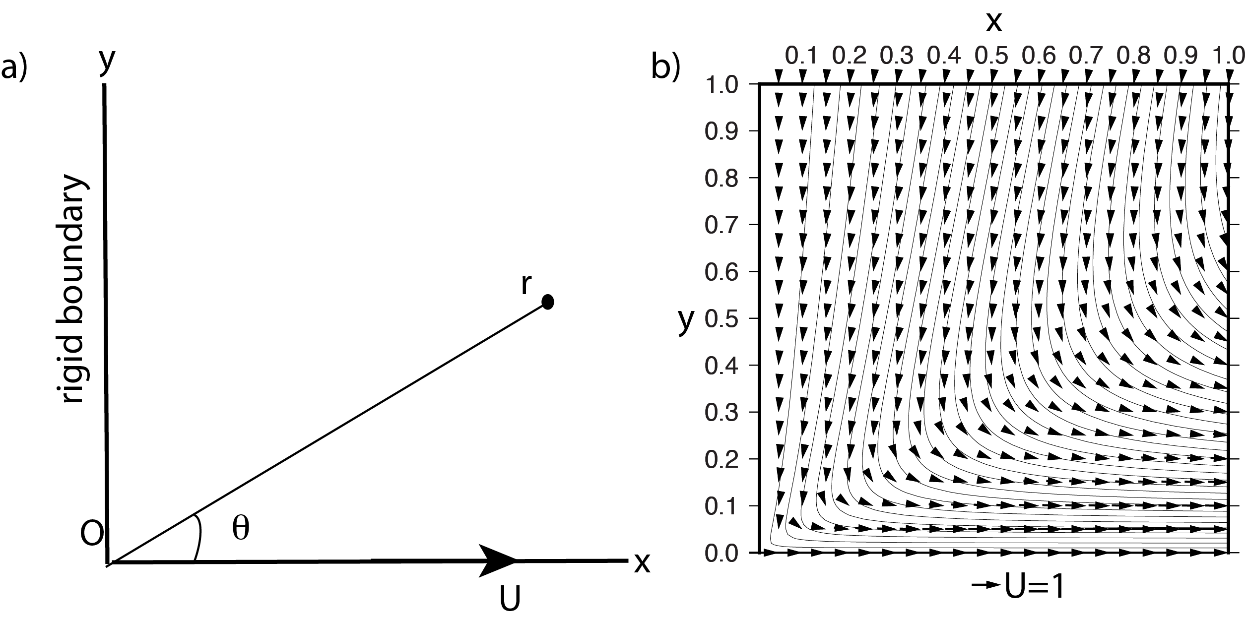Figure 1 Batchelor cornerflow geometry and solution. a) Specification of Cartesian \((x,y)\) and polar \((r,\theta)\) coordinate systems as well as boundary conditions. b) Solution for \(\psi\) (contours) and \(\vec{v}\) on geometry \(\Omega = [0,1]\times[0,1]\) with \(U=1\). Stream function contours are at arbitrary intervals.

To more easily describe the analytical solution, we consider the cornerflow geometry in Figure 1a, effectively rotating the mantle wedge by 90\(^\circ\) counterclockwise and assuming a 90\(^\circ\) angle between the wedge boundaries. In this geometry our Stokes equations can be transformed into a biharmonic equation for the stream function, \(\psi\),

(40)\[\begin{equation} \nabla^4 \psi = 0 \end{equation}\]

where \(\psi = \psi(r,\theta)\) is a function of the radius, \(r\), and angle from the \(x\)-axis, \(\theta\), related to the velocity, \(\vec{v} = \vec{v}(x, y)\) by

(41)\[\begin{align} \vec{v} = \left(\begin{array}{cc}\cos\theta & -\sin\theta \\ \sin\theta & \cos\theta\end{array}\right) \left(\begin{array}{c}\frac{1}{r}\frac{\partial\psi}{\partial\theta} \\ -\frac{\partial\psi}{\partial r}\end{array}\right) \end{align}\]

With semi-infinite \(x\) and \(y\) axes, a rigid boundary condition, \(\vec{v} = \vec{0}\), along the \(y\)-axis (the rotated “crust” at the top of the wedge), and a kinematic boundary condition on the \(x\)-axis (the ``slab’’ surface at the base of the wedge), \(\vec{v} = (U, 0)^T\), the analytical solution is found as

(42)\[\begin{equation} \psi (r, \theta)~=~ - \frac{r U }{\frac{1}{4}\pi^2-1} \left( -\frac{1}{4}\pi^2 \sin \theta + \frac{1}{2}\pi \theta \sin \theta + \theta \cos \theta \right) \end{equation}\]

Note that there was a typo in the equivalent equation (56) in Wilson & van Keken, PEPS, 2023 (II) where the negative sign above was missing.

Discretization

Since it is not possible with our numerical approach to solve the equations in a semi-infinite domain, we discretize our problem in a unit square domain with unit length in the \(x\) and \(y\) domains, as in Figure 1b. We choose different function spaces, with different shape functions, \(\vec{\omega}_j(x)\) and \(\chi_j(x)\) for the approximations of \(\vec{v}\) and \(P\) respectively, such that

(43)\[\begin{align} \vec{v} \approx \tilde{\vec{v}} &= \sum_j \omega^k_j v^k_j \\ P \approx \tilde{P} &= \sum_j \chi_j P_j \end{align}\]

where \(v^k_j\) and \(P_j\) are the values of velocity and pressure at node \(j\) respectively and the superscript \(k\) represents the spatial component of \(\vec{v}\). The discrete test functions \(\tilde{\vec{v}}_t\) and \(\tilde{P}_t\) are similarly defined. We will discuss the choice of \(\vec{\omega}_j = \omega^k_j\) and \(\chi_j\) later but simply assume that they are continuous across elements of the mesh in the following.

Boundary conditions

To match the analytical solution we apply essential Dirichlet conditions on \(\tilde{\vec{v}}\) on all four sides of the domain

(44)\[\begin{align} \tilde{\vec{v}} &= (0,0)^T && \text{on } \partial\Omega \text{ where } x=0 \\ \tilde{\vec{v}} &= (U, 0)^T && \text{on } \partial\Omega \text{ where } y=0 \\ \tilde{\vec{v}} &= \vec{v} && \text{on } \partial\Omega \text{ where } x=1 \text{ or } y = 1 \end{align}\]

Note that the first two conditions imply a discontinuity in the solution for \(\tilde{\vec{v}}\) at \((x,y)\)=\((0,0)\). The last boundary condition simply states that we apply the analytical solution at the boundaries at \(x\)=1 and \(y\)=1. One consequence of applying essential boundary conditions on \(\vec{v}\) on all sides of the domain is that \(P\) is unconstrained up to a constant value as only its spatial derivatives appear in the equations. The ability to add an arbitrary constant to the pressure is referred to as the pressure containing a null space. This makes it impossible to find a unique solution since an infinite number of pressure solutions exist. There are a number of ways to select an appropriate pressure solution. Here we arbitrarily choose one such solution by adding the condition that

(45)\[\begin{align} \tilde{P} &= 0 && \text{at } (x, y) = (0,0) \end{align}\]

which will allow a unique solution to the discrete equations to be found.

Weak form

Multiplying the momentum equation by \(\vec{v}_t\) and the continuity equation by \(P_t\), integrating (by parts) over \(\Omega\), and discretizing the test and trial functions allows the discrete matrix-vector system to be written as

(46)\[\begin{align} {\bf S} &= \left(\begin{array}{cc}{\bf K} & {\bf G} \\ {\bf D} & {\bf 0}\end{array}\right) \\ {\bf K} &= K_{i_1j_1} = \sum_k\int_{e_k} \left(\frac{\nabla\vec{\omega}_{i_1} + \nabla\vec{\omega}_{i_1}^T}{2}\right):\left(\frac{\nabla\vec{\omega}_{j_1} + \nabla\vec{\omega}_{j_1}^T}{2}\right) dx \\ {\bf G} &= G_{i_1j_2} = - \sum_k \int_{e_k} \nabla \cdot \vec{\omega}_{i_1} \chi_{j _2} dx \\ {\bf D} &= D_{i_2j_1} = - \sum_k \int_{e_k} \chi_{i_2} \nabla \cdot \vec{\omega}_{j_1} dx \\ {\bf u} &= \left({\bf v}, {\bf P}\right)^T = \left(\vec{v}_{j_1}, P_{j_2}\right)^T \\ {\bf f} &= f_i = 0 \end{align}\]

Note that all surface integrals around \(\partial\Omega\) arising from integration by parts have been dropped because the velocity solution is fully specified on all boundaries. Additionally, when integrating by parts we have used the fact that \(\nabla\vec{\omega}_{i_1}:\left(\frac{\nabla\vec{\omega}_{j_1} + \nabla\vec{\omega}_{j_1}^T}{2}\right) = \left(\frac{\nabla\vec{\omega}_{i_1} + \nabla\vec{\omega}_{i_1}^T}{2}\right):\left(\frac{\nabla\vec{\omega}_{j_1} + \nabla\vec{\omega}_{j_1}^T}{2}\right)\) to demonstrate the symmetry of \({\bf K}\). In fact, \({\bf S}\) has been made symmetric by integrating the gradient of pressure term, \(\nabla P\), by parts in and negating the continuity constraint such that \({\bf G} = {\bf D}^T\). This symmetry property can be exploited when choosing an efficient method of solving the resulting matrix equation.

An important aspect of \({\bf S}\) is that it describes a so-called “saddle point” system. The lower right block is zero, which indicates that pressure is acting in this system as a Lagrange multiplier, enforcing the constraint that the velocity is divergence free but not appearing in the continuity equation itself. Such systems require special consideration of the choice of shape functions for the discrete approximations of velocity and pressure to ensure the stability of the solution, \({\bf u}\). Several choices of so-called stable element pairs, \((\vec{\omega}_j, \chi_j)\) are available in the literature (e.g. Auricchio, 2017). Here we select the frequently used lowest-order Taylor-Hood element pair, in which \(\vec{\omega}_j\) are piecewise-quadratic and \(\chi_j\) are piecewise-linear polynomials, referred to on triangular (and tetrahedral in 3D) meshes as P2P1. This fulfills a necessary (but not sufficient) criterion for stability that the velocity has more DOFs than the pressure.