Poisson Example 1D

Authors: Cian Wilson, Peter van Keken

Description

As an introductory and simplified example we will solve the Poisson equation on a 1D domain of unit length, \(\Omega = [0,1]\), by seeking the approximate solution of

(3)\[\begin{align} -\frac{d^2 T}{dx^2} &= h % && \text{in }\Omega \end{align}\]

where we choose for this example \(h=\frac{1}{4}\pi^2 \sin\left(\frac{\pi x}{2} \right)\).

At the boundaries, \(x\)=0 and \(x\)=1, we apply as boundary conditions \begin{align} T &= 0 && \text{at } x=0 \ \frac{dT}{dx} &= 0 && \text{at } x=1 \end{align} The first boundary condition is an example of an essential or Dirichlet boundary condition where we specify the value of the solution. The second boundary condition is an example of a natural or Neumann boundary condition that can be interpreted to mean that the solution is symmetrical around \(x\)=1.

The analytical solution to the Poisson equation in 1D with the given boundary conditions and forcing function is simply

(4)\[\begin{equation} T = \sin\left(\frac{\pi x}{2}\right) \end{equation}\]

but we will still solve this numerically as a verification test of our implementation.

Weak form

The finite element method (FEM) is formulated by writing out the weak form of the equation. In the case of 1D Poisson, we multiply the equation by an arbitrary “test” function, \(T_t\), and integrate over the domain:

(5)\[\begin{equation} -\int_0^1 T_t \frac{d^2 T}{dx^2} dx = \int_0^1 T_t h dx \end{equation}\]

To lower the continuity requirements on the discrete form of \(T\) we can integrate the first term by parts giving us the weak form of the equation

(6)\[\begin{equation} \int_0^1 \frac{d T_t}{dx} \frac{d T}{dx} dx - \left[T_t \frac{dT}{dx} \right]_0^1 = \int_0^1 T_t h dx \end{equation}\]

Discretization

To discretize the equation, FEM approximates \(T\) by \(\tilde{T}\), the solution’s representation in a function space on the mesh where

(7)\[\begin{equation} \tilde{T}(\vec{x}, t) = \sum_j \phi_j(\vec{x}) T_j(t) \end{equation}\]

Here, \(T_j\) are coefficients or degrees of freedom that, as indicated, can be time-dependent if the problem is time-dependent (not the case in this example) but do not depend on space. The shape functions \(\phi_j\) are a function of space but generally independent of time. (The split of temporal and spatial dependence is typical in geodynamic applications but not required.) The index \(j\) indicates the number of the shape function on the mesh.

The mesh is constructed by dividing the domain, \(\Omega = [0,1]\), into \(n_e\) elements, chosen here to be of equal length, \(\Delta x\)=\(\frac{1}{n_e}\), with elements \(e_i\) and degrees of freedom \(T_j\) ordered from \(x\)=0 to \(x\)=1. This introduces nodal points \(x_i\), 0\(\le\)\(i\)\(\le\)\(n\) (see Figure 1).

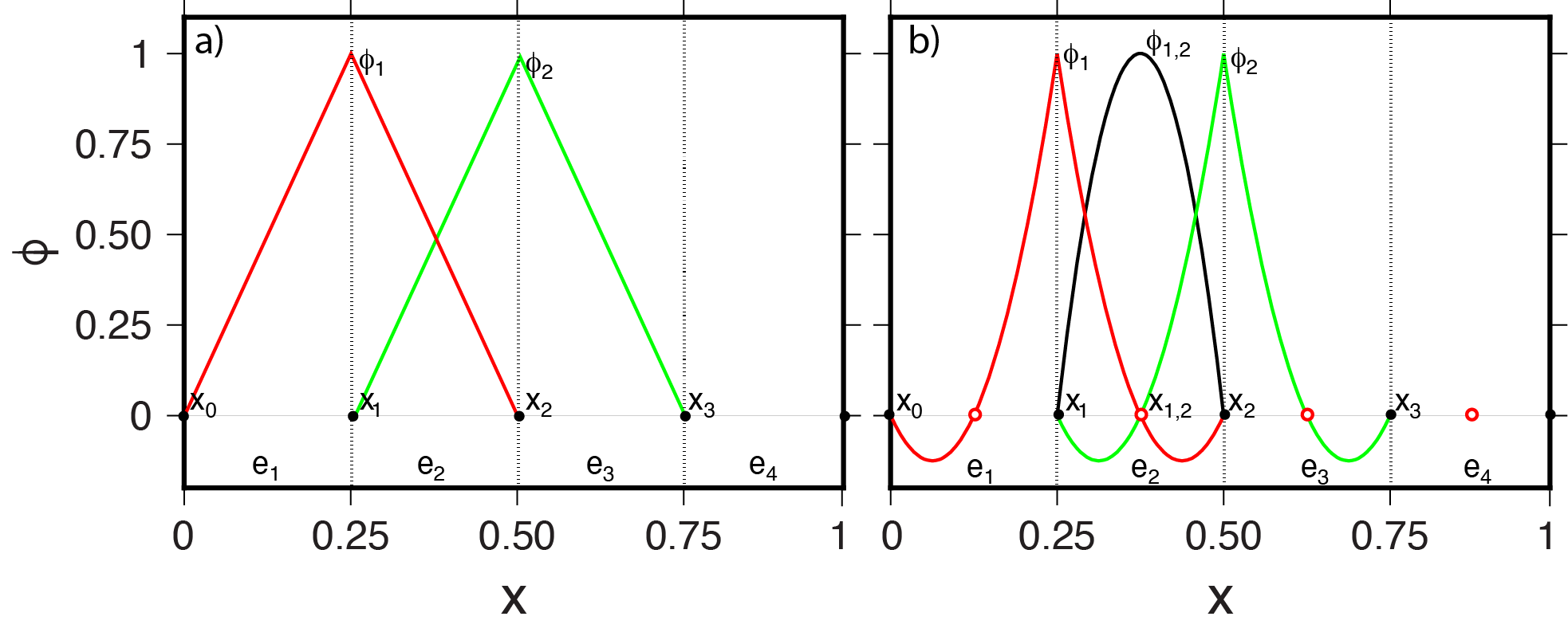Figure 1 a) Illustration of the discretization of the 1D unit domain into four elements \(e_k\) with five nodal points \(x_i\). The two linear (P1) Lagrange shape functions \(\phi_i\) are shown that are nonzero in element \(e_2\). b) Illustration of quadratic (P2) shape functions that are nonzero on element \(e_2\). The mesh still has four elements but each element now has internal nodal points (indicated by open red circles).

In this book, we will principally discuss so-called Lagrange shape functions (Figure 1) which define \(\phi_j\) as a polynomial over an element with a value of 1 at a single nodal point and a value of 0 at all other points associated with the degrees of freedom such that \(\sum_j\phi_j=1\). The shape functions can be of arbitrary order and can have various conditions on their continuity across or in between elements. We will focus principally on linear Lagrange shape functions (denoted by P1) and quadratic Lagrange shape functions (denoted by P2) that are continuous between mesh elements. Our choice of Lagrange shape functions means that \(T_j\) are the actual values of the solution. With other forms of the shape function (see, e.g., DefElement) \(T_j\) are instead interpolation weights that are used to construct the solution values.

Examining the case where the Lagrange shape functions, \(\phi_{i}\) are linear within the elements (Figure 1a), such functions within a given element \(e_i\) \((x_{i-1}\leq x \leq x_i)\), \(1\le i \le n_e\), are

(8)\[\begin{equation} \lambda_{i-1} = \frac{x_{i} - x}{\Delta x}, ~~~~~~\lambda_{i} = \frac{x-x_{i-1}}{\Delta x} \end{equation}\]

The functions \(\lambda_{j}\) are zero for all elements except \(e_{j}\) and \(e_{j+1}\) (\(\forall e_i\)\(\notin\)\(\{e_{j}, e_{j+1}\}\)). Since they fit the definition of linear Lagrange functions and we can write \(\phi_i=\lambda_i\) and within a given element \(e_i\) (\(x_{i-1} \leq x \leq x_i\)) we can construct the interpolated approximate solution for \(\tilde{T}\) using

(9)\[\begin{equation} \tilde{T}(x) = T_{i-1} \phi_{i-1} (x) + T_{i} \phi_{i} (x) \end{equation}\]

In the case of quadratic Lagrange shape functions, \(\phi_{i}\) are quadratic within the elements (Figure 1b). Note that each element now has an internal nodal point such that the number of nodal points for the fixed number of elements increases by nearly a factor of two compared to the linear P1 function space (Figure 1a). Within an element \(e_i\) (\(x_{i-1}\)\(\leq\)\(x\)\(\leq\)\(x_i\)) there are three shape functions that are of quadratic form

(10)\[\begin{align} \phi_{i-1} ~ & =~ \frac{2}{\Delta x^2} (x - x_i)(x - x_{i-1,i}) =~ 2 \lambda_{i-1} ( \lambda_{i-1} - \tfrac{1}{2} ) \\ \phi_{i-1,i} ~ & =~ \frac{-4}{\Delta x^2} (x - x_{i-1})(x - x_i) = 4\lambda_{i-1}\lambda_i \\ \phi_{i} ~ & =~ \frac{2}{\Delta x^2} (x - x_{i-1})(x - x_{i-1,i}) = 2 \lambda_i ( \lambda_i - \tfrac{1}{2} ) \end{align}\]

with \(\lambda_i\) and \(\lambda_{i-1}\) defined as before. We have used the notation \(\phi_{i-1,i}\) to identify the internal Lagrange polynomial centered in element \(e_i\) on the new internal nodal point \(x_{i-1,i}\). This also makes explicit the relation between the P1 nodal points and the mesh cell edge nodal points (also called vertices) of the P2 elements and clarifies the relation between P1 and P2 shape functions.

The test functions \(T_t\) can be independent of the functions that span the function space of the trial function, but in the widely used Galerkin approach the test functions are restricted to be in the same function space such that

(11)\[\begin{equation} \tilde{T}_t(\vec{x}, t) = \sum_i\phi_i(\vec{x}) T_{ti}(t) \end{equation}\]

Since the method is valid for all \(\tilde{T}_t\) we can dispense with the test function values at the DOFs, \(T_{ti}\) and, through substitution of \(T = \tilde{T}\) and \(T_t = \tilde{T}_t\) write the discrete weak form as

(12)\[\begin{equation} \sum_j\int_0^1 \frac{d \phi_i}{dx} \frac{d \phi_j}{dx} dx T_j - \sum_j\left[\phi_i \frac{d\phi_j}{dx} \right]_0^1 T_j = \int_0^1 \phi_i h dx, \quad\quad i = 1,\ldots, n \end{equation}\]

The second term can be dropped because we require \(\frac{d\tilde{T}}{dx} = 0\) at \(x=1\) and the solution at \(x=0\) (\(i=0\)) is known (\(T_0=0\))

(13)\[\begin{equation} \sum_j\int_0^1 \frac{d \phi_i}{dx} \frac{d \phi_j}{dx} dx T_j = \int_0^1 \phi_i h dx, \quad\quad i = 1,\ldots, n \end{equation}\]

Matrix equation

Given a domain with \(n\) DOFs such that \(i,j=1, \ldots, n\), the discrete weak form can be assembled into a matrix-vector system of the form

(14)\[\begin{equation} {\bf S} {\bf u} = {\bf f} \end{equation}\]

where \(\bf{S}\) is a \(n \times n\) matrix, \(\bf{f}\) is the right-hand side vector of length \(n\) and \(\bf{u}\) is the solution vector of values at the DOFs

(15)\[\begin{align} {\bf S} &= S_{ij} = \int_0^1 \frac{d\phi_i}{dx} \frac{d\phi_j}{dx} ~dx \\ {\bf f} &= f_i = \int_0^1 \phi_i h ~dx \\ {\bf u} &= {\bf T} = T_j \end{align}\]

where \({\bf T}\) has components \(T_j\) that define the continuous approximate solution

(16)\[\begin{equation} \tilde{T}(x) = \sum_{j=1}^n \phi_j(x) T_j \end{equation}\]

and \(T_0 = 0\).

When using linear Lagrange shape functions these integrals can be easily evaluated by noting that the derivatives of \(\phi_i\) in element \(e_i\) are simply

(17)\[\begin{equation} \frac{d \phi_{i-1}}{dx} = -\frac{1}{\Delta x}, ~~~~~~\frac{d \phi_{i}}{dx} = \frac{1}{\Delta x} \end{equation}\]

which allows for easy evaluation of the matrix and vector coefficients

(18)\[\begin{equation} \frac{1}{\Delta x^2}\left(\begin{array}{cccccccc} 2 & -1 & 0 & \cdots & 0 & 0 & 0 \\ -1 & 2 & -1 & \cdots & 0 & 0 & 0 \\ \vdots & \vdots & \vdots & & \vdots & \vdots & \vdots \\ 0 & 0 & 0 & \cdots & -1 & 2 & -1 \\ 0 & 0 & 0 & \cdots & 0 & -1 & 1\end{array}\right) \left(\begin{array}{c} T_1\\T_2\\\vdots\\T_{n-1}\\T_{n}\end{array}\right) = \left(\begin{array}{c} \int h \phi_1 dx \\ \int h \phi_2 dx \\ \vdots\\ \int h \phi_{n-1} dx\\ \int h \phi_n dx\end{array}\right) \end{equation}\]

The integral in the right-hand side vector \({\bf f}\) can be found analytically or through numerical integration. The matrix may look familiar to those acquainted with finite difference approximations to the 1D Poisson equation where \(d^2T/dx^2\) is approximated by second-order central finite differences. The matrix rows repeat triples (-1,2,-1) to form a tridiagonal symmetric matrix for which (very) efficient solution methods exist. For a sufficiently large mesh the matrix is also sparse (most entries are zero) because the shape functions are compact – all shape functions other than \(\phi_{i-1}\) and \(\phi_{i}\) are zero within element \(e_i\) (for a linear Lagrange shape function, P1).

Note that in the P2 case, the nonzero values of a quadratic Lagrange shape function may extend beyond their immediate neighbor nodes and can be positive or negative depending on where its nodal point is located within an element. Note also that the shape functions will also connect more nodal points to the central nodal point – which suggests the matrix changes form to have more entries per row than in the case of the P1 based matrix. In addition the matrix will have more rows since there are more nodal points for the same number of elements. Clearly the use of higher order elements comes at a greater computational cost since it is more expensive to solve a larger algebraic system.