Batchelor Cornerflow Example#
Authors: Cameron Seebeck, Cian Wilson
Description#
As a reminder we are seeking the approximate velocity and pressure solution of the Stokes equation
in a unit square domain, \(\Omega = [0,1]\times[0,1]\).
We apply strong Dirichlet boundary conditions for velocity on all four boundaries
and an additional point constraint on pressure
to remove its null space.
Implementation#
This example was presented by Wilson & van Keken, 2023 using FEniCS v2019.1.0 and TerraFERMA, a GUI-based model building framework that also uses FEniCS v2019.1.0. Here we reproduce these results using the latest version of FEniCS, FEniCSx.
Preamble#
We start by loading all the modules we will require and initializing our plotting preferences through pyvista.
from mpi4py import MPI
import dolfinx as df
import dolfinx.fem.petsc
import numpy as np
import ufl
import matplotlib.pyplot as pl
import basix
import sys, os
basedir = ''
if "__file__" in globals(): basedir = os.path.dirname(__file__)
sys.path.append(os.path.join(basedir, os.path.pardir, 'python'))
import utils
import pyvista as pv
if __name__ == "__main__" and "__file__" in globals():
    pv.OFF_SCREEN = True
import pathlib
if __name__ == "__main__":
    output_folder = pathlib.Path(os.path.join(basedir, "output"))
    output_folder.mkdir(exist_ok=True, parents=True)
Solution#
We start by defining the analytical solution
where \(\psi = \psi(r,\theta)\) is a function of the radius, \(r\), and angle from the \(x\)-axis, \(\theta\)
We describe this solution using UFL in the python function v_exact_batchelor.
def v_exact_batchelor(mesh, U=1):
    """
    A python function that returns the exact Batchelor velocity solution
    using UFL.
    Parameters:
    * mesh - the mesh on which we wish to define the coordinates for the solution
    * U    - convergence speed of lower boundary (defaults to 1)
    """
    # Define the coordinate systems
    x = ufl.SpatialCoordinate(mesh)
    theta = ufl.atan2(x[1],x[0])

    # Define the derivative to the streamfunction psi
    d_psi_d_r = -U*(-0.25*ufl.pi**2*ufl.sin(theta) \
                    +0.5*ufl.pi*theta*ufl.sin(theta) \
                    +theta*ufl.cos(theta)) \
                    /(0.25*ufl.pi**2-1)
    d_psi_d_theta_over_r = -U*(-0.25*ufl.pi**2*ufl.cos(theta) \
                               +0.5*ufl.pi*ufl.sin(theta) \
                               +0.5*ufl.pi*theta*ufl.cos(theta) \
                               +ufl.cos(theta) \
                               -theta*ufl.sin(theta)) \
                               /(0.25*ufl.pi**2-1)

    # Rotate the solution into Cartesian and return
    return ufl.as_vector([ufl.cos(theta)*d_psi_d_theta_over_r + ufl.sin(theta)*d_psi_d_r, \
                          ufl.sin(theta)*d_psi_d_theta_over_r - ufl.cos(theta)*d_psi_d_r])
We then declare a python function solve_batchelor that contains a complete description of the discrete Stokes equation problem.
This function follows much the same flow as described in previous examples
we describe the unit square domain \(\Omega = [0,1]\times[0,1]\) and discretize it into \(2 \times\)
ne\(\times\)netriangular elements or cells to make ameshwe declare finite elements for velocity and pressure using Lagrange polynomials of degree
p+1andprespectively and use these to declare the mixed function space,Vof the coupled problem and the sub function spaces,V_v,V_vx,V_vy, andV_p, for velocity, \(x\) velocity, \(y\) velocity, and pressure respectivelyusing the mixed function space we declare trial,
v_aandp_a, and test,v_tandp_t, functions for the velocity and pressure respectivelywe define a list of Dirichlet boundary conditions,
bcs, including velocity boundary conditions on all four sides and a constraint on the pressure in the lower left corner of the domainwe describe the discrete weak forms,
Sandf, that will be used to assemble the matrix \(\mathbf{S}\) and vector \(\mathbf{f}\)we solve the matrix problem using a linear algebra back-end and return the solution
def solve_batchelor(ne, p=1, U=1):
    """
    A python function to solve a two-dimensional corner flow
    problem on a unit square domain.
    Parameters:
    * ne - number of elements in each dimension
    * p  - polynomial order of the pressure solution (defaults to 1)
    * U  - convergence speed of lower boundary (defaults to 1)
    """
    # Describe the domain (a unit square)
    # and also the tessellation of that domain into ne
    # equally spaced squared in each dimension, which are
    # subduvided into two triangular elements each
    mesh = df.mesh.create_unit_square(MPI.COMM_WORLD, ne, ne)

    # Define velocity and pressure elements
    v_e = basix.ufl.element("Lagrange", mesh.basix_cell(), p+1, shape=(mesh.geometry.dim,))
    p_e = basix.ufl.element("Lagrange", mesh.basix_cell(), p)

    # Define the mixed element of the coupled velocity and pressure
    vp_e = basix.ufl.mixed_element([v_e, p_e])

    # Define the mixed function space
    V = df.fem.functionspace(mesh, vp_e)

    # Define velocity and pressure sub function spaces
    V_v, _ = V.sub(0).collapse()
    V_vx, _ = V_v.sub(0).collapse()
    V_vy, _ = V_v.sub(1).collapse()
    V_p, _ = V.sub(1).collapse()

    # Define the trial functions for velocity and pressure
    v_a, p_a = ufl.TrialFunctions(V)
    # Define the test functions for velocity and pressure
    v_t, p_t = ufl.TestFunctions(V)

    # Declare a list of boundary conditions
    bcs = []

    # Define the location of the left boundary and find the velocity DOFs
    def boundary_left(x):
        return np.isclose(x[0], 0)
    dofs_v_left = df.fem.locate_dofs_geometrical((V.sub(0), V_v), boundary_left)
    # Specify the velocity value and define a Dirichlet boundary condition
    zero_v = df.fem.Function(V_v)
    zero_v.x.array[:] = 0
    bcs.append(df.fem.dirichletbc(zero_v, dofs_v_left, V.sub(0)))

    # Define the location of the bottom boundary and find the velocity DOFs
    # for x velocity (0) and y velocity (1) separately
    def boundary_base(x):
        return np.isclose(x[1], 0)
    dofs_vx_base = df.fem.locate_dofs_geometrical((V.sub(0).sub(0), V_vx), boundary_base)
    dofs_vy_base = df.fem.locate_dofs_geometrical((V.sub(0).sub(1), V_vy), boundary_base)
    # Specify the value of the x component of velocity and define a Dirichlet boundary condition
    U_vx = df.fem.Function(V_vx)
    U_vx.x.array[:] = U
    bcs.append(df.fem.dirichletbc(U_vx, dofs_vx_base, V.sub(0).sub(0)))
    # Specify the value of the y component of velocity and define a Dirichlet boundary condition
    zero_vy = df.fem.Function(V_vy)
    zero_vy.x.array[:] = 0.0
    bcs.append(df.fem.dirichletbc(zero_vy, dofs_vy_base, V.sub(0).sub(1)))

    # Define the location of the right and top boundaries and find the velocity DOFs
    def boundary_rightandtop(x):
        return np.logical_or(np.isclose(x[0], 1), np.isclose(x[1], 1))
    dofs_v_rightandtop = df.fem.locate_dofs_geometrical((V.sub(0), V_v), boundary_rightandtop)
    # Specify the exact velocity value and define a Dirichlet boundary condition
    exact_v = df.fem.Function(V_v)
    # Interpolate from a UFL expression, evaluated at the velocity interpolation points
    exact_v.interpolate(df.fem.Expression(v_exact_batchelor(mesh, U=U), V_v.element.interpolation_points()))
    bcs.append(df.fem.dirichletbc(exact_v, dofs_v_rightandtop, V.sub(0)))

    # Define the location of the lower left corner of the domain and find the pressure DOF there
    def corner_lowerleft(x):
        return np.logical_and(np.isclose(x[0], 0), np.isclose(x[1], 0))
    dofs_p_lowerleft = df.fem.locate_dofs_geometrical((V.sub(1), V_p), corner_lowerleft)
    # Specify the arbitrary pressure value and define a Dirichlet boundary condition
    zero_p = df.fem.Function(V_p)
    zero_p.x.array[:] = 0.0
    bcs.append(df.fem.dirichletbc(zero_p, dofs_p_lowerleft, V.sub(1)))

    # Define the integrals to be assembled into the stiffness matrix
    K = ufl.inner(ufl.sym(ufl.grad(v_t)), ufl.sym(ufl.grad(v_a))) * ufl.dx
    G = -ufl.div(v_t)*p_a*ufl.dx
    D = -p_t*ufl.div(v_a)*ufl.dx
    S = K + G + D

    # Define the integral to the assembled into the forcing vector
    # which in this case is just zero so arbitrarily use the pressure test function
    zero = df.fem.Constant(mesh, df.default_scalar_type(0.0))
    f = zero*p_t*ufl.dx

    # Compute the solution (given the boundary conditions, bcs)
    problem = df.fem.petsc.LinearProblem(S, f, bcs=bcs, \
                                         petsc_options={"ksp_type": "preonly", \
                                                        "pc_type": "lu", \
                                                        "pc_factor_mat_solver_type": "mumps"})
    u_i = problem.solve()

    # Extract the velocity and pressure solutions from the coupled problem
    v_i = u_i.sub(0).collapse()
    p_i = u_i.sub(1).collapse()

    return v_i, p_i
We can now numerically solve the equations using, e.g., 10 elements in each dimension and piecewise linear polynomials for pressure.
if __name__ == "__main__":
    ne = 10
    p = 1
    U = 1
    v, p = solve_batchelor(ne, p=p, U=U)
    v.name = "Velocity"
main
Note that this code block starts with if __name__ == "__main__": to prevent it from being run unless being run as a script or in a Jupyter notebook. This prevents unecessary computations when this code is used as a python module.
And use some utility functions (see ../python/utils.py) to plot the velocity glyphs.
if __name__ == "__main__":
    plotter = utils.plot_mesh(v.function_space.mesh, gather=True, show_edges=True, style="wireframe")
    utils.plot_vector_glyphs(v, plotter=plotter, gather=True, factor=0.3)
    utils.plot_show(plotter)
    utils.plot_save(plotter, output_folder / 'batchelor_solution.png')
    comm = v.function_space.mesh.comm
    if comm.size > 1:
        # if we're running in parallel (e.g. from a script) then save an image per process as well
        plotter_p = utils.plot_mesh(v.function_space.mesh, show_edges=True, style="wireframe")
        utils.plot_vector_glyphs(v, plotter=plotter_p, factor=0.3)
        utils.plot_show(plotter_p)
        utils.plot_save(plotter_p, output_folder / 'batchelor_solution_p{:d}.png'.format(comm.rank,))
Testing#
Error analysis#
We can quantify the error in cases where the analytical solution is known by taking the L2 norm of the difference between the numerical and exact solutions.
def evaluate_error(v_i, U=1):
    """
    A python function to evaluate the l2 norm of the error in
    the two dimensional Batchelor corner flow problem given the known analytical
    solution.
    """
    # Define the exact solution (in UFL)
    ve = v_exact_batchelor(v_i.function_space.mesh, U=U)

    # Define the error as the squared difference between the exact solution and the given approximate solution
    l2err = df.fem.assemble_scalar(df.fem.form(ufl.inner(v_i - ve, v_i - ve)*ufl.dx))
    l2err = v_i.function_space.mesh.comm.allreduce(l2err, op=MPI.SUM)**0.5

    # Return the l2 norm of the error
    return l2err
Convergence test#
if __name__ == "__main__":
    # Open a figure for plotting
    fig = pl.figure()
    ax = fig.gca()

    # Set the convergence velocity
    U = 1
    # List of polynomial orders to try
    ps = [1, 2]
    # List of resolutions to try
    nelements = [10, 20, 40, 80]
    # Keep track of whether we get the expected order of convergence
    test_passes = True
    # Loop over the polynomial orders
    for p in ps:
        # Accumulate the errors
        errors_l2_a = []
        # Loop over the resolutions
        for ne in nelements:
            # Solve the 2D Batchelor corner flow problem
            v_i, p_i = solve_batchelor(ne, p=p, U=U)
            # Evaluate the error in the approximate solution
            l2error = evaluate_error(v_i, U=U)
            # Print to screen and save if on rank 0
            if v_i.function_space.mesh.comm.rank == 0:
                print('ne = ', ne, ', l2error = ', l2error)
            errors_l2_a.append(l2error)

        # Work out the order of convergence at this p
        hs = 1./np.array(nelements)/p

        # Write the errors to disk
        if v_i.function_space.mesh.comm.rank == 0:
            with open(output_folder / 'batchelor_convergence_p{}.csv'.format(p), 'w') as f:
                np.savetxt(f, np.c_[nelements, hs, errors_l2_a], delimiter=',',
                       header='nelements, hs, l2errs')

        # Fit a line to the convergence data
        fit = np.polyfit(np.log(hs), np.log(errors_l2_a),1)
        if v_i.function_space.mesh.comm.rank == 0:
            print("***********  order of accuracy p={}, order={}".format(p,fit[0]))

        # log-log plot of the L2 error
        ax.loglog(hs,errors_l2_a,'o-',label='p={}, order={:.2f}'.format(p,fit[0]))

        # Test if the order of convergence is as expected (first order)
        test_passes = test_passes and abs(fit[0]-1) < 0.1

    # Tidy up the plot
    ax.set_xlabel('h')
    ax.set_ylabel('||e||_2')
    ax.grid()
    ax.set_title('Convergence')
    ax.legend()

    # Write convergence to disk
    if v_i.function_space.mesh.comm.rank == 0:
        fig.savefig(output_folder / 'batchelor_convergence.pdf')

        print("***********  convergence figure in output/batchelor_convergence.pdf")

    # Check if we passed the test
    assert(test_passes)
ne =  10 , l2error =  0.021921089471662054
ne =  20 , l2error =  0.010960435556187281
ne =  40 , l2error =  0.005480211135211691
ne =  80 , l2error =  0.0027401051388766555
***********  order of accuracy p=1, order=1.0000050785210133
ne =  10 , l2error =  0.012877716729227353
ne =  20 , l2error =  0.006438858695195689
ne = 40 , l2error = 0.0032194293512690826
ne =  80 , l2error =  0.0016097146756369792
***********  order of accuracy p=2, order=0.9999999771201509
*********** convergence figure in output/batchelor_convergence.pdf
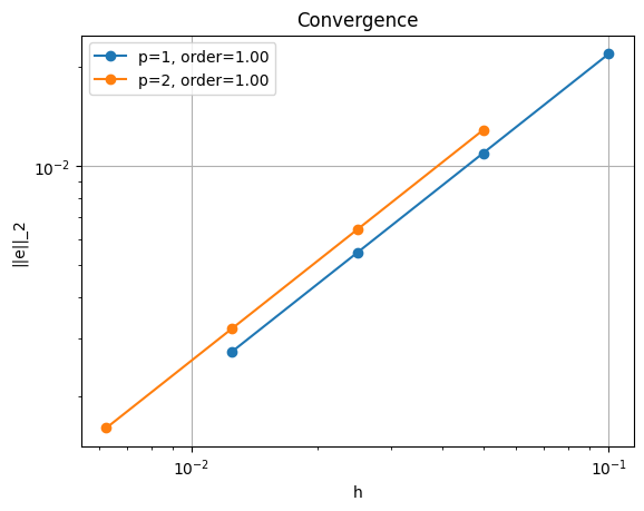
Solving the equations on a series of successively finer meshes and comparing the resulting solution to the analytical result using the error metric
shows linear rather than quadratic convergence, regardless of the polynomial order we select for our numerical solution.
This first-order convergence rate is lower than would be expected for piecewise quadratic or piecewise cubic velocity functions (recall that the velocity is one degree higher than the specified pressure polynomial degree). This drop in convergence is caused by the boundary conditions at the origin being discontinuous, which cannot be represented in the selected function space and results in a pressure singularity at that point. This is an example where convergence analysis demonstrates suboptimal results due to our inability to represent the solution in the selected finite element function space.
Finish up#
Convert this notebook to a python script (making sure to save first)
if __name__ == "__main__" and "__file__" not in globals():
    from ipylab import JupyterFrontEnd
    app = JupyterFrontEnd()
    app.commands.execute('docmanager:save')
    !jupyter nbconvert --NbConvertApp.export_format=script --ClearOutputPreprocessor.enabled=True batchelor.ipynb
[NbConvertApp] Converting notebook batchelor.ipynb to script
[NbConvertApp] Writing 16274 bytes to batchelor.py